
Computer Vision - Part 8: One-Stage Detectors — YOLO and SSD
Computer Vision — Part 8: One-Stage Detectors — YOLO and SSD
Two-stage detectors such as Faster R-CNN are accurate, but they are too slow for many real-time tasks. One-stage detectors predict boxes and classes in a single forward pass. They trade a small amount of accuracy for a large speed gain.
This part explains the two most influential one-stage families: YOLO (You Only Look Once) and SSD (Single Shot MultiBox Detector).
1. One-stage vs two-stage detectors
| Step | Two-stage (Faster R-CNN) | One-stage (YOLO/SSD) |
|---|---|---|
| 1 | Run CNN once → feature map | Run CNN once → feature maps |
| 2 | Region Proposal Network proposes boxes | Predict boxes directly from feature maps |
| 3 | Crop regions, classify and refine | Classify and refine in one pass |
Because the second stage is removed, one-stage detectors can run at 30, 60, or even hundreds of frames per second.
The disadvantage is that one-stage detectors may struggle more with small or densely packed objects. They also balance more tasks at once in a single loss.
2. YOLO — You Only Look Once
YOLO reframed detection as a single regression problem. Instead of proposing regions and classifying them, YOLO divides the image into a grid and, in one shot, predicts boxes for every grid cell.
YOLOv1 idea
1. Divide the image into an S × S grid (e.g. 7 × 7).
2. Each grid cell predicts:
   - B bounding boxes (default B = 2)
   - a confidence score for each box
   - a class probability distribution
3. During inference, combine confidence and class probability to get the final score for each box.
An object is only assigned to a grid cell if its centroid falls inside that cell — even if its bounding box leaks into neighbouring cells. This one-centroid-one-cell rule is what stops the same object from being registered twice by different cells.
The grid size S is a speed/accuracy dial. A coarse grid (e.g. 3 × 3) trains and runs faster but misses fine detail and struggles with small or closely-packed objects. A finer grid (e.g. 7 × 7 or higher) is more sensitive to detail and more accurate, at the cost of a larger output tensor and slower training and inference. The right choice depends on how small and how densely packed the objects in the target dataset are.

For every grid cell, the output tensor looks like:
[ x, y, w, h, confidence, c1, c2, ..., cC ]
(x, y)is the centre of the box relative to the grid cell.(w, h)is the width and height relative to the whole image.confidenceisPr(object) × IoU.c1...cCare class probabilities.
The full prediction is a 3-D tensor:
shape = (S, S, B * 5 + C)
For S = 7, B = 2, and C = 20:
shape = (7, 7, 30)
That is the entire output of the network for one image.
Multiple objects in the same grid cell
A single grid cell can only “own” one prediction slot per box. But what if two objects — say a cyclist and their bike — have centroids that fall in the same cell? A plain grid cell cannot register both at once.
This is exactly the problem anchor boxes solve. Instead of predicting one box per cell, YOLO predicts A boxes per cell, one per anchor shape (a tall anchor for the cyclist, a wide anchor for the motorbike, for example). Each anchor gets its own confidence, box offsets, and class vector, and they are concatenated into a single output:
output length per cell = C + 5 * A
where A is the number of anchor boxes tried at that cell. The person is matched to whichever anchor shape overlaps it best, the motorbike is matched to a different anchor, and both can be reported out of the same cell without colliding.
At inference, the network never predicts a box from scratch — it predicts a confidence, an objectness/class score, and small offsets for each tiled anchor, then uses those offsets to nudge the anchor towards the real object. Anchors that don’t match any training class are dropped, the rest are filtered by confidence score, and non-maximum suppression picks the best survivor per object.
Loss in YOLOv1
The YOLOv1 loss has several parts:
L = λ_coord * L_coord    (error in box centres and sizes)
  + λ_noobj * L_conf_noobj  (confidence for empty cells)
  + L_conf_obj              (confidence for cells with objects)
  + L_cls                   (classification error)
λ_coord is usually 5 to make the network pay more attention to getting boxes right. λ_noobj is usually 0.5 because most cells do not contain an object.
How YOLO works step by step
- Image → CNN backbone: The image passes through a CNN to produce a feature map.
- Feature map → grid predictions: A few convolutional layers turn the feature map into an
S × S × (B * 5 + C)tensor. - Decode boxes: For each cell, turn
(x, y, w, h)into real image coordinates. - Compute scores: Multiply
confidenceby each class probability to getconfidence × class_probfor every box and class. - Threshold: Keep boxes whose score is above a threshold, such as
0.5. - Non-Maximum Suppression: Remove overlapping duplicates.
3. Decoding a YOLO prediction
Suppose a grid cell predicts:
x = 0.6, y = 0.4, w = 0.5, h = 0.3, confidence = 0.8
dog = 0.7, cat = 0.2, bicycle = 0.1
If the cell is at column i = 2 and row j = 3 in a 7 × 7 grid on a 448 × 448 image:
cell_width  = 448 / 7 = 64
cell_height = 448 / 7 = 64

cell_top_left_x = i * cell_width  = 2 * 64 = 128
cell_top_left_y = j * cell_height = 3 * 64 = 192

box_centre_x = cell_top_left_x + x * cell_width  = 128 + 0.6 * 64 = 166.4
box_centre_y = cell_top_left_y + y * cell_height = 192 + 0.4 * 64 = 217.6

box_width  = w * image_width  = 0.5 * 448 = 224
box_height = h * image_height = 0.3 * 448 = 134.4
The final box, in corner format, is:
x1 = 166.4 - 224 / 2 = 54.4
y1 = 217.6 - 134.4 / 2 = 150.4
x2 = 166.4 + 224 / 2 = 278.4
y2 = 217.6 + 134.4 / 2 = 284.8
The score for class “dog” for this box is:
score = confidence × P(dog) = 0.8 × 0.7 = 0.56
That score is compared against the threshold to decide whether to keep the box.
4. YOLO output analysis
A YOLO model produces a large tensor. The post-processing steps convert that tensor into clean boxes, labels, and confidence scores.
Step 1: confidence and class scores
For each predicted box, the network gives:
confidence— how sure it is that an object exists hereclass logits— raw scores for each class
During inference, the class logits are usually converted to probabilities with softmax or sigmoid depending on the YOLO version.
For YOLOv3 and later, classes are predicted independently with sigmoid, so the same box can belong to multiple classes if desired.
Step 2: score thresholding
Most predictions are garbage. A threshold, typically 0.25 to 0.5, removes boxes with low confidence.
Step 3: Non-Maximum Suppression (NMS)
One real object often triggers several grid cells and anchors. NMS keeps the highest-scoring box and removes boxes that overlap it too much.
1. Sort all boxes by score.
2. Take the box with the highest score as the current box.
3. Remove all boxes whose IoU with the current box is above a threshold (e.g. 0.45).
4. Repeat with the next highest-scoring box until no boxes remain.
NMS is what turns thousands of raw predictions into a small number of clean detections.
5. SSD — Single Shot MultiBox Detector
SSD has the same one-stage philosophy as YOLO, but it uses feature maps at multiple scales instead of one grid.
Architecture: convolutional predictors
The SSD head is more than one small filter. After a base network such as VGG-16, it adds six extra convolutional layers. These layers make the feature maps smaller and deeper — like looking at a thumbnail that is packed with more labels. Because of this:
- The early, high-resolution layers keep small details, so they are better for finding small objects.
- The later, smaller layers see a bigger area at once, so they are better for finding large objects.
In short, SSD uses these layers like a set of magnifying glasses at different zoom levels.
Multi-scale feature maps
A CNN creates several feature maps as it processes an image. Earlier layers are large and contain fine details, which help detect small objects. Later layers are small and contain high-level patterns, which help detect large objects.
Layer 1  →  large feature map  →  small anchors  →  detect small objects
Layer 2  →  medium feature map →  medium anchors
Layer 3  →  small feature map   →  large anchors  →  detect large objects
SSD places anchors on many layers, then predicts class and offsets for every anchor.
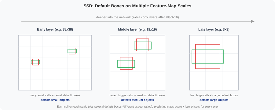
Default boxes
SSD calls its anchor boxes default boxes. These are pre-made box shapes of different sizes and aspect ratios. At every location on a feature map, SSD tries 4 or 6 of these boxes. Each default box is a starting guess, and the network asks two questions:
- Is this box on an object, or on background? (class score)
- If it is on an object, how should I shift or resize the box to fit? (box offsets)
Matching strategy
SSD matches each ground-truth box to the default box with the highest IoU. It also matches every default box whose IoU with any ground truth is above 0.5. This means one object can be matched to multiple default boxes, giving the network more positive examples.
Localization and confidence loss
SSD’s total loss has two parts:
- Localization loss — for positive matches, this measures how far the predicted box is from the ground-truth box. It tells the network how to shift and resize the box.
- Confidence loss — for every positive match, the network is encouraged to be confident about the correct object class. For every negative match, it is encouraged to be confident about the background / “no object” class. The final loss is the sum of these two.
Hard negative mining
Because most default boxes are background, positives are rare. SSD uses hard negative mining: it selects the background boxes with the highest loss, rather than using all of them. This keeps the training set balanced and focused on the most confusing negatives.
6. YOLO vs SSD
| Feature | YOLO | SSD |
|---|---|---|
| Grid/anchors | Single grid in v1; multiple scales and anchors from v2 onward | Multiple feature-map scales with default boxes |
| Speed | Very fast, especially newer versions | Fast, slightly slower than modern YOLO |
| Small objects | Struggled in early versions; improved in YOLOv3+ | Generally better because of multi-scale features |
| Loss emphasis | Strong weight on coordinate loss | Balanced classification and localisation loss |
| Post-processing | NMS on grid cells | NMS on all default boxes |
Both models are fully convolutional, so they can be run on images of different sizes.
7. Code: simulate a YOLO-style output and decode it
import numpy as np

def decode_yolo_cell(i, j, S, pred, image_size):
    """
    pred = [x, y, w, h, confidence, ...class scores...]
    Returns box in corner format [x1, y1, x2, y2] and score for class 0.
    """
    cell_w = image_size[1] / S
    cell_h = image_size[0] / S

    x = pred[0]
    y = pred[1]
    w = pred[2]
    h = pred[3]
    confidence = pred[4]
    class_scores = pred[5:]

    cx = i * cell_w + x * cell_w
    cy = j * cell_h + y * cell_h

    box_w = w * image_size[1]
    box_h = h * image_size[0]

    x1 = cx - box_w / 2
    y1 = cy - box_h / 2
    x2 = cx + box_w / 2
    y2 = cy + box_h / 2

    best_class = np.argmax(class_scores)
    best_score = class_scores[best_class]
    final_score = confidence * best_score

    return [x1, y1, x2, y2], final_score, best_class

S = 7
image_size = (448, 448)

# Random prediction for cell (2, 3)
pred = np.array([0.6, 0.4, 0.5, 0.3, 0.8, 0.7, 0.2, 0.1])
box, score, cls = decode_yolo_cell(2, 3, S, pred, image_size)
print(f"Decoded box: {box}, class {cls}, score {score:.2f}")
8. Summary
- One-stage detectors perform classification and localisation in a single network pass. They are fast and suitable for real-time applications.
- YOLO divides the image into a grid and predicts boxes, confidence, and class probabilities directly from the grid cells.
- A YOLO prediction is decoded by converting cell-relative
(x, y, w, h)into image coordinates and multiplying confidence by class probability. - NMS removes duplicate boxes for the same object.
- SSD uses anchors on multiple feature-map scales, which improves detection of small objects.
- SSD uses hard negative mining to balance the huge number of background boxes.
- YOLO and SSD are both fully convolutional and have influenced nearly all modern real-time detectors.