
Part 9: Convolutional Neural Networks (CNNs) - A Friendly Guide
Part 9: Convolutional Neural Networks (CNNs) — A Friendly Guide
This guide is for someone who is starting from zero. You do not need to know computer vision before reading this.
In the earlier deep learning parts, we used a spam email example. We converted one email into a small list of numbers such as suspicious words, links, known sender, and message length. That worked because the input was already simple.
Images are different.
A photo is not a short list. A photo is a large grid of numbers. A color photo has three grids: red, green, and blue. A computer does not see a cat, a dog, an eye, or a wheel. It only sees pixel numbers.
So the big question is:
How can a neural network turn raw pixel numbers into a useful answer like “cat” or “dog”?
A Convolutional Neural Network, or CNN, is a neural network designed especially for images. It learns visual patterns step by step:
Pixels → edges → textures → parts → object → prediction
This guide builds that idea slowly, one concept at a time.
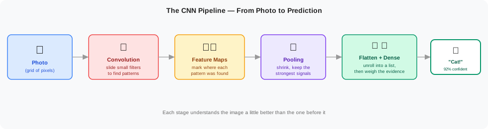
Memory trick: A CNN reads an image like a person understands a face: first small details, then shapes, then the whole object.
1. What problem are we solving?
Imagine we want a model to look at a photo and answer:
Cat or dog?
For a human, this feels easy. You look at the image and notice ears, eyes, fur, nose shape, and body shape.
For a computer, the image is just numbers:
Pixel brightness, pixel brightness, pixel brightness, ...
A small image might be 32 × 32 pixels. A real image might be 224 × 224 pixels. If the image is color, every pixel has 3 values:
- Red brightness
- Green brightness
- Blue brightness
So a 224 × 224 color image has:
224 × 224 × 3 = 150,528 numbers
That is much bigger than the 5-number spam example.
A CNN exists because images have two important properties:
- Nearby pixels are related. Pixels next to each other may form an edge, corner, eye, or texture.
- The same pattern can appear anywhere. A cat ear might be at the top-left, top-right, or center of a photo.
A CNN is built around these two facts.
2. Why not use a normal fully connected network?
Before CNNs, let us first understand the simpler option: a fully connected layer.
A fully connected layer means:
Every input number is connected to every neuron in the next layer.
A connection is just a weight the model must learn.
Simple example: 5 numbers
In the spam example, one email had only 5 input numbers:
[ suspicious words, links, known sender, capitals, length ]
If the next layer has 3 neurons, then each neuron looks at all 5 numbers:
Neuron 1 uses 5 weights
Neuron 2 uses 5 weights
Neuron 3 uses 5 weights
So the total is:
5 inputs × 3 neurons = 15 weights
That is small and manageable.
Now compare that with an image
A 224 × 224 color image has:
224 × 224 × 3 = 150,528 numbers
So an image is not 5 numbers. It is 150,528 numbers.
If we use a fully connected layer, each neuron must look at all 150,528 numbers.
Problem 1: too many weights
Suppose the next layer has 1,000 neurons.
One neuron needs:
150,528 weights
Because it looks at all 150,528 input numbers.
Now multiply that by 1,000 neurons:
150,528 × 1,000 = 150,528,000 weights
So just the first layer needs more than 150 million weights.
That is too large for a beginner-friendly image model. It uses a lot of memory, takes more computation, and can easily memorize training images instead of learning useful visual patterns.
Problem 2: no understanding of nearby pixels
A fully connected layer treats every pixel as just another number.
It does not automatically know that nearby pixels are related.
But images depend on nearby pixels:
dark pixel next to bright pixel → maybe an edge
several edges together          → maybe a curve
curves and textures together    → maybe an ear or eye
So location matters. Pixels next to each other often create meaningful visual patterns.
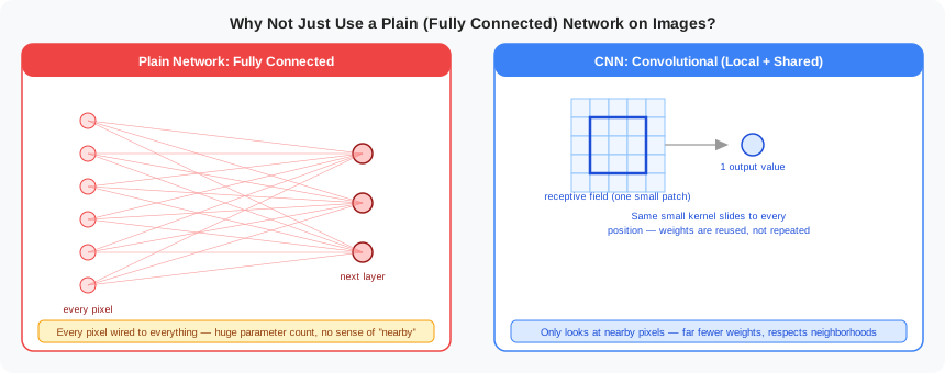
A CNN solves both problems by looking at a small patch of the image instead of the whole image at once.
It uses a small window, checks one patch, then slides to the next patch, then the next.
That sliding operation is called convolution.
Memory trick: Fully connected means every pixel talks to every neuron. Convolution means one small window moves around and reuses the same pattern detector everywhere.
3. The first key idea: a small pattern detector
Before learning the word convolution, learn the simple idea behind it.
Imagine a CNN is looking at a picture using a small magnifying glass.
- The input is the picture.
- The filter is the magnifying glass.
- The padding is the extra border around the picture.
- The stride is how far the magnifying glass jumps each time.
3.1 Input: the picture
The input is the image given to the CNN. A small grayscale image might look like this:
1   2   3   4   5
6   7   8   9  10
11 12 13 14 15
16 17 18 19 20
21 22 23 24 25
This is a 5 × 5 image:
5 rows
5 columns
Think of each number as one tiny pixel. A real photo has many more pixels and usually three color channels — red, green, and blue — but the idea is the same.
3.2 Filter: the small magnifying glass
A filter is a small box that looks at only part of the image at one time.
A filter is also called a kernel. The two words mean the same thing. We will keep using both because PyTorch uses the word kernel in code, but in plain English they are identical.
A common filter size is 3 × 3. It can look at 9 pixels at once:
[ 1  0 -1 ]
[ 1  0 -1 ]
[ 1  0 -1 ]
This filter is good at detecting a vertical edge. It compares the left side of the patch to the right side.
Now place it on the top-left of a small image:
Image patch          Filter
[ 1  2  3 ]          [ 1  0 -1 ]
[ 0  1  2 ]    ×     [ 1  0 -1 ]
[ 3  1  0 ]          [ 1  0 -1 ]
Multiply each image value by the matching filter value:
(1 × 1) + (2 × 0) + (3 × -1)
+ (0 × 1) + (1 × 0) + (2 × -1)
+ (3 × 1) + (1 × 0) + (0 × -1)
Add all the results:
1 + 0 - 3 + 0 + 0 - 2 + 3 + 0 + 0 = -1
That single number -1 becomes one value in the output feature map.
A filter may learn to detect:
| Pattern | What it finds |
|---|---|
| Vertical edges | Sides of an object |
| Horizontal edges | Top or bottom boundary |
| Corners | Where two edges meet |
| Curves | Circular shapes |
| Textures | Fur, grass, or fabric |
| Complex features | Eyes, wheels, or faces |
The programmer does not usually choose the filter values by hand. During training, the CNN learns values such as:
[ 0.2  0.7  0.1]
[-0.4  0.3  0.6]
[ 0.1 -0.5 -0.2]
These numbers are weights. Backpropagation adjusts them so the filter becomes useful.
3.3 Stride: how far the filter moves
Stride tells us how many pixels the filter moves each time.
Stride = 1
The filter moves one pixel at a time:
Position 1:  [F F F . .]
             [F F F . .]
             [F F F . .]

Position 2:  [. F F F .]
             [. F F F .]
             [. F F F .]

Position 3:  [. . F F F]
             [. . F F F]
             [. . F F F]
It checks many positions, so the output is larger.
Stride = 2
The filter jumps two pixels at a time:
Position 1:  [F F F . .]
             [F F F . .]
             [F F F . .]

Position 2:  [. . F F F]
             [. . F F F]
             [. . F F F]
It checks fewer positions, so the output is smaller.
| Stride | Movement | Output size |
|---|---|---|
S = 1 |
Move 1 pixel | Larger |
S = 2 |
Jump 2 pixels | Smaller |
S = 3 |
Jump 3 pixels | Much smaller |
3.4 Padding: adding a border
Padding means adding extra pixels around the outside of the image. Usually the extra pixels are zeros.
A 3 × 3 image:
1 2 3
4 5 6
7 8 9
With padding = 1:
0 0 0 0 0
0 1 2 3 0
0 4 5 6 0
0 7 8 9 0
0 0 0 0 0
Padding gives the filter space to look at the edge pixels. Without padding, the filter cannot place its centre on the outside edge, and the output becomes smaller after every convolution.
| Padding | What happens |
|---|---|
padding = 0 |
No extra border. Output shrinks. |
padding = 1 |
Add 1 pixel border. Output can stay the same size with a 3 × 3 filter. |
padding = 2 |
Add 2 pixel border. Used for larger filters. |
3.5 Put everything together
Suppose we have:
Input:   5 × 5
Filter:  3 × 3
Padding: 0
Stride:  1
The filter starts here:
[F F F . .]
[F F F . .]
[F F F . .]
[. . . . .]
[. . . . .]
Then moves right:
[. F F F .]
[. F F F .]
[. F F F .]
[. . . . .]
[. . . . .]
Then right again:
[. . F F F]
[. . F F F]
[. . F F F]
[. . . . .]
[. . . . .]
There are 3 horizontal positions. The filter also moves downward into 3 vertical positions. So the output is:
3 × 3
This matches the exact formula you will see later:
Output size = ((N - F + 2P) / S) + 1
For this example:
Output size = ((5 - 3 + 2×0) / 1) + 1
            = (2 / 1) + 1
            = 3
Example from your question
For a 32 × 32 image, a 3 × 3 filter, padding = 0, and stride = 1:
Output size = ((32 - 3 + 2×0) / 1) + 1
            = 29 + 1
            = 30
So the output feature map is 30 × 30.
3.6 Simple memory table
| Term | Kid-friendly meaning |
|---|---|
| Input | The whole picture |
| Filter | A small magnifying glass looking for patterns |
| Padding | An extra border around the picture |
| Stride | How far the magnifying glass moves |
Easy sentence:
The filter moves across the input using a stride, while padding protects the edges.
The patch currently being looked at is called the receptive field.
4. What is convolution?
Convolution means sliding a filter — also called a kernel — across an image and producing a score at every location.
The process is:
Take a small patch
→ multiply patch values by filter (kernel) weights
→ add the results
→ write one output number
→ slide to the next patch
→ repeat
One filter (kernel) produces one new grid of numbers. That grid is called a feature map.
If the filter (kernel) detects vertical edges, the feature map becomes bright where vertical edges exist. If it detects curves, the feature map becomes bright where curves exist.
In PyTorch
A convolution layer is written with nn.Conv2d:
import torch
import torch.nn as nn

image = torch.randn(1, 3, 224, 224)

conv_layer = nn.Conv2d(
    in_channels=3,
    out_channels=64,
    kernel_size=3,
    padding=1,
    stride=1
)

feature_maps = conv_layer(image)
print(feature_maps.shape)  # torch.Size([1, 64, 224, 224])
Here is what each part means:
| Code | Meaning |
|---|---|
1 |
One image in the batch |
3 |
Three color channels: red, green, blue |
224, 224 |
Image height and width |
in_channels=3 |
The input has 3 channels |
out_channels=64 |
Learn 64 different filters (kernels) |
kernel_size=3 |
Each filter (kernel) looks at a 3 × 3 area |
padding=1 |
Add a small border so the output size stays controlled |
stride=1 |
Move the filter (kernel) one pixel at a time |
Why 64 output channels?
out_channels=64 means the layer has 64 different filters (kernels).
Each filter (kernel) learns to detect a different visual pattern. One might detect vertical edges. Another might detect horizontal edges. Another might detect color changes. Another might detect small curves.
So one image goes in, but 64 feature maps come out:
1 image → 64 pattern maps
For a color image, each filter (kernel) must look through all 3 input channels. So a 3 × 3 filter (kernel) over an RGB image actually has:
3 × 3 × 3 = 27 weights
One filter (kernel) produces one feature map. Sixty-four filters (kernels) produce sixty-four feature maps.
Recap
| Term | Simple meaning |
|---|---|
| Kernel / filter | A small learned pattern detector |
| Receptive field | The small image patch currently being checked |
| Convolution | Sliding the detector over the image |
| Feature map | A grid showing where a pattern was found |
| Output channels | Number of feature maps produced |
5. Why do we need ReLU after convolution?
A convolution produces raw scores. Some scores are positive. Some are negative.
But if we only stack weighted sums on top of weighted sums, the model remains too simple. It cannot learn complex visual decisions well.
So after convolution, CNNs usually apply an activation function called ReLU.
ReLU means Rectified Linear Unit.
Its rule is simple:
\[\text{ReLU}(x) = \max(0, x)\]In plain English:
positive number → keep it
negative number → change it to 0
Example:
relu = nn.ReLU()
print(relu(torch.tensor([2.4, -0.7, 1.3])))
# tensor([2.4, 0.0, 1.3])
Why is this useful?
ReLU acts like a switch. If a pattern is useful, let the signal continue. If the signal is negative, turn it off. This helps the CNN build more complex patterns layer by layer.
Memory trick: ReLU is a gate. Positive signals pass through; negative signals are stopped.
6. What is a feature map?
A feature map is the output produced by one filter (kernel) after it scans the image.
Think of it like a highlighted copy of the image.
If the filter (kernel) searches for vertical edges, the feature map highlights places where vertical edges were found. If it searches for curves, the feature map highlights curves.
A CNN does not use just one filter (kernel). It uses many filters (kernels).
| Filter (kernel) may learn to detect | Feature map lights up where |
|---|---|
| Vertical edge | Vertical lines appear |
| Horizontal edge | Horizontal lines appear |
| Color change | Color changes sharply |
| Curve | Curved shapes appear |
| Texture | Repeated patterns appear |
The next convolution layer does not return to the original image. It looks at the feature maps from the previous layer.
That is how the CNN builds understanding:
First layers: edges and colors
Middle layers: textures and simple shapes
Later layers: object parts like eyes, ears, wheels, faces
Memory trick: A feature map is like a highlighter mark showing where one visual clue was found.
7. Padding: why add a border around the image?
When a filter (kernel) slides over an image, it has trouble at the edges.
A 3 × 3 filter (kernel) needs a full 3 × 3 patch. At the border, there are not enough surrounding pixels unless we do something special.
Without padding, the output becomes smaller after each convolution.
Padding means adding extra pixels around the image before applying convolution.
The most common type is zero padding:
add a border of zeros around the image
This helps control the output size.
VGG16 uses padding=1 for its 3 × 3 convolutions. That keeps the height and width the same after convolution. The image only shrinks later during pooling.
Memory trick: Padding is like adding a blank picture frame around the image so the filter (kernel) can scan the edges too.
8. Pooling: why shrink the feature maps?
After convolution and ReLU, the CNN may have many large feature maps. Processing all of them can be expensive.
Pooling shrinks feature maps while keeping the strongest signals.
The most common type is max pooling.
Max pooling looks at a small block, often 2 × 2, and keeps only the largest number.
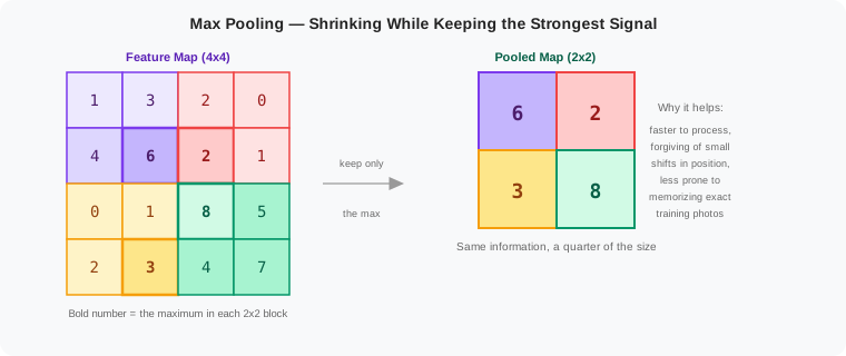
Example:
pool_layer = nn.MaxPool2d(kernel_size=2, stride=2)

pooled = pool_layer(feature_maps)
print(pooled.shape)  # torch.Size([1, 64, 112, 112])
If the input feature map is 224 × 224, max pooling with kernel_size=2 and stride=2 reduces it to 112 × 112.
Why do this?
- Less work: smaller feature maps are faster to process.
- Less noise: keep the strongest signal and ignore weaker details.
- Small movement tolerance: if an eye moves slightly left or right, the model can still notice it.
Pooling has no learned weights and no bias. It is only a fixed operation.
Memory trick: Max pooling is like summarizing four nearby clues by keeping the strongest one.
9. The CNN pattern so far
A beginner-friendly CNN usually repeats this pattern:
Convolution → ReLU → Pooling
Each part has a job:
| Step | Job |
|---|---|
| Convolution | Search for visual patterns |
| ReLU | Keep useful positive signals and turn off negative ones |
| Pooling | Shrink the map while keeping strong signals |
After one block, the image becomes a set of smaller feature maps.
After many blocks, the CNN has learned richer features:
Image pixels
→ simple feature maps
→ smaller feature maps
→ richer feature maps
→ object clues
Now the CNN needs to turn those clues into a final answer.
10. From feature maps to a decision
After several convolution blocks, the CNN no longer has a normal image. It has a stack of feature maps.
Those feature maps might contain signals like:
- strong edge pattern
- possible ear shape
- possible eye shape
- fur-like texture
- dog-nose-like shape
But the final classifier expects a simple list of numbers.
So we use flatten.
Flatten turns a stack of grids into one long vector:
many 2D feature maps → one long list of numbers
flatten = nn.Flatten()
flat_vector = flatten(pooled)  # shape: [1, 64*112*112]
Then a dense classifier makes the final decision:
classifier = nn.Sequential(
    nn.Linear(64 * 112 * 112, 128),
    nn.ReLU(),
    nn.Linear(128, 2),
    nn.Softmax(dim=1)
)

output = classifier(flat_vector)
print(output)  # e.g. tensor([[0.92, 0.08]]) → 92% cat, 8% dog
The final 2 means there are two classes:
class 0 = cat
class 1 = dog
Softmax turns raw scores into probabilities that add up to 1.
Example:
[0.92, 0.08] = 92% cat, 8% dog
The highest probability becomes the prediction.
11. Exact formulas, explained gently
This section is optional on the first read. The main idea is simple: formulas help answer two practical questions:
1. What will the output shape be?
2. How many learnable numbers does this layer store?
If you understand those two questions, the formulas become less scary.
Formula 1: output size
When a filter (kernel) slides across an image, it creates a new grid of numbers.
That new grid is the output feature map.
The size of this new grid depends on how the filter (kernel) moves:
- No padding: the filter (kernel) cannot fully cover the border pixels, so the output usually becomes smaller.
- With padding: we add a border around the image, so the output can stay the same size.
- Bigger stride: the filter (kernel) jumps more pixels at a time, so the output becomes smaller faster.
So this formula answers one simple question:
If my input image is this size, what size will the output feature map be?
For one side of the image, such as height or width:
\[\text{Output size} = \left\lfloor \frac{N - F + 2P}{S} \right\rfloor + 1\]Read the formula like this:
| Symbol | Simple meaning | Example |
|---|---|---|
N |
Original input size | 224 pixels wide |
F |
Filter/kernel size | 3 × 3 kernel means F = 3 |
P |
Padding added on each side | 1 pixel border |
S |
Stride, how far the filter (kernel) moves | 1 pixel at a time |
Why + 2P? Padding is added to both sides. If P = 1, we add 1 pixel on the left and 1 pixel on the right, so the total added width is 2.
For VGG16’s common convolution:
N = 224
F = 3
P = 1
S = 1
Step by step:
Output size = ((224 - 3 + 2×1) / 1) + 1
            = ((224 - 3 + 2) / 1) + 1
            = (223 / 1) + 1
            = 224
So a 224 × 224 image stays 224 × 224 after this convolution.
That is why VGG16 can apply convolution without shrinking the image. The shrinking happens later during max pooling.
Formula 2: convolution parameter count
A convolution layer stores learned numbers. These are the model’s memory.
Each filter has:
filter (kernel) height × filter (kernel) width × input channels
For example, one 3 × 3 filter (kernel) looking at an RGB image has:
3 × 3 × 3 = 27 weights
Each filter also has one bias.
So the formula is:
\[\text{Parameters} = (\text{number of filters}) \times (F \times F \times \text{input channels}) + \text{number of filters}\]The final + number of filters means one bias per filter.
Example: first VGG16 convolution
The first VGG16 convolution uses:
64 filters (kernels)
3 × 3 filter (kernel)
3 input channels: red, green, blue
One filter has:
3 × 3 × 3 = 27 weights
Sixty-four filters have:
64 × 27 = 1,728 weights
Each filter has one bias:
64 biases
Total:
1,728 weights + 64 biases = 1,792 parameters
Example: deeper VGG16 convolution
A deeper VGG16 layer may use:
512 filters (kernels)
3 × 3 filter (kernel)
512 input channels
One filter has:
3 × 3 × 512 = 4,608 weights
All filters together have:
512 × 4,608 = 2,359,296 weights
Add one bias for each of the 512 filters:
2,359,296 + 512 = 2,359,808 parameters
This is much larger because the layer receives 512 input channels instead of 3.
Recap
| Question | Formula |
|---|---|
| What is the output size? | $\left\lfloor \dfrac{N-F+2P}{S} \right\rfloor + 1$ |
| How many conv parameters? | filters × (F × F × input channels) + filters |
| How many dense parameters? | inputs × outputs + outputs |
Memory trick: Output-size formula tells you the new image size. Parameter-count formula tells you how much the layer remembers.
12. A real CNN: VGG16
Now we can understand a real CNN architecture.
VGG16 is a famous image classification CNN. It is useful for learning because its structure is simple and repetitive.
VGG16 mostly repeats this pattern:
Conv 3 × 3 → ReLU → Conv 3 × 3 → ReLU → MaxPool
It uses:
- 13 convolution layers to extract image features
- 5 max pooling layers to shrink feature maps
- 3 dense layers to make the final classification
The name VGG16 means it has 16 learnable weight layers:
13 convolution layers + 3 dense layers = 16 weight layers
Pooling layers are not counted because they have no learned weights.
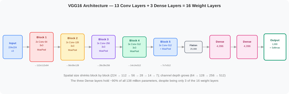
VGG16 starts with a 224 × 224 × 3 image.
Read this shape as:
224 = height
224 = width
3   = color channels: red, green, blue
As the image moves through the network:
- Convolution layers change the number of channels. For example, 64 filters produce 64 output channels.
- Pooling layers shrink height and width. For example,
224 × 224becomes112 × 112. - Deeper layers keep more pattern maps. The network remembers many kinds of clues while the spatial size becomes smaller.
A shape like 112 × 112 × 128 means:
112 pixels high
112 pixels wide
128 feature maps / channels
The table below follows the image as it travels through VGG16. You do not need to memorize the whole table. Read it as a story: size goes down, channels go up, and parameters are stored only in convolution and dense layers.
| # | Layer | Output shape | Parameters |
|---|---|---|---|
| 1 | Conv 3x3, 64 filters | 224 x 224 x 64 | 1,792 |
| 2 | Conv 3x3, 64 filters | 224 x 224 x 64 | 36,928 |
| — | MaxPool 2x2 | 112 x 112 x 64 | 0 |
| 3 | Conv 3x3, 128 filters | 112 x 112 x 128 | 73,856 |
| 4 | Conv 3x3, 128 filters | 112 x 112 x 128 | 147,584 |
| — | MaxPool 2x2 | 56 x 56 x 128 | 0 |
| 5 | Conv 3x3, 256 filters | 56 x 56 x 256 | 295,168 |
| 6 | Conv 3x3, 256 filters | 56 x 56 x 256 | 590,080 |
| 7 | Conv 3x3, 256 filters | 56 x 56 x 256 | 590,080 |
| — | MaxPool 2x2 | 28 x 28 x 256 | 0 |
| 8 | Conv 3x3, 512 filters | 28 x 28 x 512 | 1,180,160 |
| 9 | Conv 3x3, 512 filters | 28 x 28 x 512 | 2,359,808 |
| 10 | Conv 3x3, 512 filters | 28 x 28 x 512 | 2,359,808 |
| — | MaxPool 2x2 | 14 x 14 x 512 | 0 |
| 11 | Conv 3x3, 512 filters | 14 x 14 x 512 | 2,359,808 |
| 12 | Conv 3x3, 512 filters | 14 x 14 x 512 | 2,359,808 |
| 13 | Conv 3x3, 512 filters | 14 x 14 x 512 | 2,359,808 |
| — | MaxPool 2x2 | 7 x 7 x 512 | 0 |
| — | Flatten | 25,088 | 0 |
| 14 | Dense | 4,096 | 102,764,544 |
| 15 | Dense | 4,096 | 16,781,312 |
| 16 | Dense + Softmax | 1,000 | 4,097,000 |
| Total | 138,357,544 |
Two important observations:
- Pooling shrinks width and height.
224 → 112 → 56 → 28 → 14 → 7. - Convolution increases channels. The network moves from 64 feature maps to 128, then 256, then 512.
- Dense layers contain most parameters. The first dense layer alone has over 102 million parameters.
Why is the first dense layer so large?
Before the dense layer, VGG16 has:
7 × 7 × 512 = 25,088 numbers
The first dense layer connects those 25,088 numbers to 4,096 neurons:
25,088 × 4,096 + 4,096 = 102,764,544 parameters
So VGG16 teaches an important lesson: convolution layers are efficient because they reuse small filters across the image, while dense layers become expensive because every input connects to every output.
13. Optional deep dive: only the details you need
You can understand CNNs without going very deep into every detail. But a few extra ideas make the whole picture clearer.
Deep dive 1: Who decides the number of filters?
The person designing the model chooses the number of filters. This is part of the model architecture.
For example:
nn.Conv2d(3, 64, kernel_size=3)
Read it as:
3  input channels come in
64 filters are created
64 feature maps come out
The model does not automatically decide to use 64 filters. The human designer chooses 64. Then training learns the values inside those 64 filters.
Why choose more filters?
More filters mean the layer can look for more kinds of patterns.
16 filters  → small/simple model
64 filters  → more pattern detectors
512 filters → many pattern detectors, but expensive
Common choices are 16, 32, 64, 128, 256, and 512 filters. More filters can make the model stronger, but they also require more memory, more computation, and more training data.
Deep dive 2: What does a filter learn?
At the beginning of training, filter values are random. They do not yet detect anything useful.
During training, the model makes predictions, measures mistakes with a loss function, and backpropagation adjusts the filter weights. After seeing many images, some filters become useful detectors.
A simple mental model:
random filter
→ many training examples
→ many small weight updates
→ useful pattern detector
Different layers tend to learn different levels of patterns:
early filters → edges, colors, corners
middle filters → textures, curves, simple shapes
later filters → eyes, wheels, faces, object parts
So a filter is not hand-coded to detect an eye or an edge. It learns useful values from data.
Deep dive 3: Why do channels increase while image size decreases?
CNNs usually follow this pattern:
height and width go down
number of channels goes up
Example from VGG16:
224 × 224 × 64
112 × 112 × 128
56 × 56 × 256
28 × 28 × 512
14 × 14 × 512
7 × 7 × 512
This can feel strange at first: why make the image smaller but increase channels?
Think of the network as moving from location detail to meaning detail.
Early layers need large width and height because they are asking:
Where are the edges?
Where are the corners?
Where are the color changes?
Later layers do not need exact pixel-level location as much. They are asking:
Is there an eye-like pattern?
Is there a wheel-like pattern?
Is there a face-like pattern?
So the network keeps fewer positions but stores more types of clues at each position.
Simple way to think about it:
early layers: many locations, simple clues
later layers: fewer locations, richer clues
Deep dive 4: What is learned and what is not learned?
Not every CNN operation learns weights.
| Layer | Learns weights? | Job |
|---|---|---|
| Convolution | Yes | Learn visual pattern detectors |
| ReLU | No | Turn negative values into zero |
| Max pooling | No | Shrink feature maps |
| Flatten | No | Rearrange grids into a list |
| Dense layer | Yes | Combine clues for final decision |
| Softmax | No | Convert scores into probabilities |
The model’s memory is mainly stored in convolution weights, convolution biases, dense weights, and dense biases.
14. Try it yourself: a mini CNN in PyTorch
Here is a small CNN with the same basic pattern, but much smaller than VGG16.
It works with fake 32 × 32 color images and predicts two classes.
import torch
import torch.nn as nn

class MiniCNN(nn.Module):
    def __init__(self):
        super().__init__()
        self.features = nn.Sequential(
            nn.Conv2d(3, 16, kernel_size=3, padding=1), nn.ReLU(),
            nn.MaxPool2d(2, 2),
            nn.Conv2d(16, 32, kernel_size=3, padding=1), nn.ReLU(),
            nn.MaxPool2d(2, 2),
        )
        self.classifier = nn.Sequential(
            nn.Flatten(),
            nn.Linear(32 * 8 * 8, 64), nn.ReLU(),
            nn.Linear(64, 2),
            nn.Softmax(dim=1)
        )

    def forward(self, x):
        x = self.features(x)
        return self.classifier(x)

model = MiniCNN()
image = torch.randn(1, 3, 32, 32)
prediction = model(image)
print(prediction)  # e.g. tensor([[0.63, 0.37]])
The flow is:
32 × 32 RGB image
→ Conv + ReLU
→ Pool to 16 × 16
→ Conv + ReLU
→ Pool to 8 × 8
→ Flatten
→ Dense classifier
→ probability for each class
To use real images, you would add training data, a loss function, and an optimizer, just like the earlier deep learning tutorials.
15. Final summary
A CNN is not magic. It is a careful chain of simple operations:
Image
→ convolution finds local patterns
→ ReLU keeps useful signals
→ feature maps remember where patterns appeared
→ pooling shrinks the maps
→ deeper layers combine simple patterns into richer patterns
→ flatten turns maps into a list
→ dense layers make the final decision
→ softmax gives probabilities
| Concept | Simple meaning |
|---|---|
| Convolution | Slide a small pattern detector across the image |
| Kernel / filter | The small learned detector |
| Receptive field | The image patch currently being checked |
| Feature map | A grid showing where one pattern was found |
| ReLU | Keep positive signals, turn negative signals into zero |
| Padding | Add a border so convolution can handle edges |
| Pooling | Shrink the map while keeping strong signals |
| Flatten | Turn grids into one long list |
| Dense layer | Combine all final clues into a decision |
| Softmax | Convert final scores into probabilities |
16. Memory tricks recap
| Concept | Memory trick |
|---|---|
| Convolution | A flashlight scanning one small patch at a time |
| Kernel / filter | A mini stencil hunting for one pattern |
| ReLU | A gate that blocks negative numbers |
| Feature map | A highlighted report showing where a pattern was found |
| Padding (zero) | A blank picture frame border |
| Pooling | Keep the strongest clue from a small area |
| Flatten | Unrolling a folded map into one straight strip |
| Dense layer | A detective weighing every clue before the verdict |
| Softmax | Turning raw scores into percentages that add up to 100% |
Previous: Part 8: Deep Learning Cheat Sheet · Next: Part 10: Advanced Convolutional Neural Networks