
Part 10: Advanced Convolutional Neural Networks - A Friendly Guide
Part 10: Advanced Convolutional Neural Networks — A Friendly Guide
In Part 9, we learned the basic CNN flow:
Image
→ Convolution
→ ReLU
→ Pooling
→ Feature maps
→ Flatten
→ Dense layers
→ Prediction
That is enough to understand the foundation.
But real-world CNNs often need a few extra ideas to work well:
- How do we make CNNs deeper without making training fail?
- How do we stop a CNN from memorizing training images?
- How do we reuse a model that was already trained on millions of images?
- Why do modern CNNs often avoid huge dense layers?
This guide answers those questions in simple English.
1. Why do we need advanced CNN ideas?
A small CNN can learn simple images.
But real images are messy:
- Different lighting
- Different backgrounds
- Different object sizes
- Object partly hidden
- Camera angle changes
- Noise and blur
A cat may appear close, far away, sideways, bright, dark, or partly behind a chair.
A basic CNN may struggle with that.
Advanced CNN ideas help the model become:
| Problem | Helpful idea |
|---|---|
| Model memorizes training images | Dropout, data augmentation |
| Training becomes unstable | Batch normalization |
| Deep network becomes hard to train | Residual connections |
| Dense layers become too large | Global average pooling |
| Not enough training data | Transfer learning |
We will go one by one.
2. Deeper CNNs: why not just add more layers?
A deeper CNN can learn richer patterns.
Early layers  → edges and colors
Middle layers → textures and shapes
Later layers  → object parts
Very deep layers → whole object concepts
So it sounds like we should just add more convolution layers.
But deeper networks create new problems.
Problem 1: harder training
When a network becomes very deep, the learning signal must travel through many layers during backpropagation.
Sometimes the early layers receive weak or confusing updates.
This can make the model train slowly or poorly.
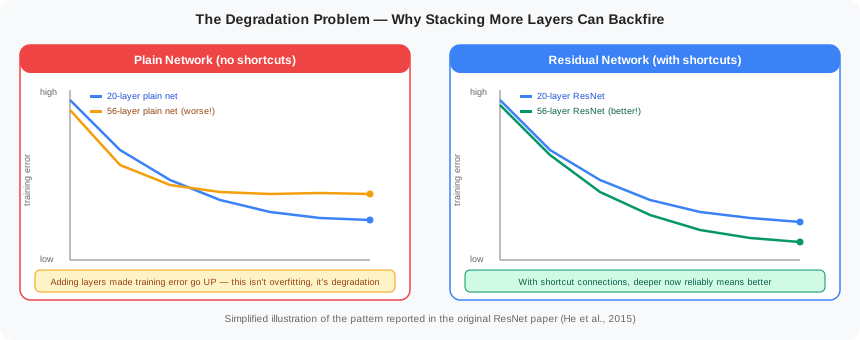
Researchers saw this happen directly: when they compared a 20-layer plain network to a 56-layer plain network, the 56-layer network ended up with higher training error — not just worse results on new images, but worse results even on the images it was trained on. This is called the degradation problem, and it’s the main reason later architectures added the residual connections covered in section 7.
Problem 2: overfitting
A bigger model has more learnable weights.
If the dataset is small, the model may memorize the training images instead of learning general patterns.
Memorizing = works well on training images, fails on new images
Learning   = works well on new images too
Advanced CNN techniques exist mainly to fix these two problems.
3. Overfitting: the model memorizes instead of learning
Imagine training a CNN with 100 cat images and 100 dog images.
If the model is too powerful, it may memorize details like:
- This exact cat photo has a blue sofa
- This dog photo has grass in the background
- This cat image has a specific shadow
Then it may fail on a new cat photo with a different background.
That is overfitting.
A good model should learn reusable patterns:
cat-like ears
cat-like eyes
fur texture
face shape
body shape
not just the exact training photos.
4. Data augmentation: create more variety
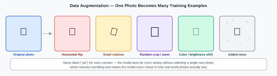
Data augmentation means creating modified copies of training images so the model sees more variety without collecting new data.
Why augmentation is needed
Imagine you have imbalanced training data:
1000 cat images
1000 dog images
  50 truck images
The model will see cats and dogs very often, but trucks barely at all.
It may learn cats and dogs well, but fail on trucks.
Augmentation helps:
50 original truck images
→ each image is transformed multiple ways
→ now you have many effective truck examples
Augmentation is also useful when you simply do not have enough total data.
Why copy-paste is not augmentation
Just copying and pasting images does not help.
copy + paste = same information, just repeated
The model sees the same pixels repeated and learns nothing new.
Real augmentation applies small changes that make the image look slightly different:
original image
→ rotate 15 degrees
→ now a slightly different sample with new angle information
The model has to generalize to that variation, which makes it stronger.
Three categories of augmentation
1. Geometric transformations
These change the shape, position, or orientation of the image.
| Example | What the model learns |
|---|---|
| Rotation | Object can appear tilted |
| Crop | Object may appear at different positions |
| Flip | Object can face left or right |
| Zoom in or out | Object can appear larger or smaller |
| Elastic distortion | Object can look slightly warped |
2. Color space transformations
These change the colors or brightness of the image.
| Example | What the model learns |
|---|---|
| Brightness change | Lighting conditions vary |
| Contrast change | Image can look washed out or sharp |
| Hue or saturation shift | Colors can shift slightly |
| RGB channel adjustment | Color balance can change |
3. Filtering
These apply visual effects to the image.
| Example | What the model learns |
|---|---|
| Blur | Images may not always be sharp |
| Add noise | Images may have small random variations |
Advanced: GAN-based augmentation
Generative adversarial networks can create entirely new synthetic images.
GAN generates new, realistic-looking images
→ add those images to the training set
→ model sees more variety
This is more complex and usually not needed for beginners, but useful for very small datasets.
The label stays the same
For all augmentation types, the label does not change.
original truck image      → label: truck
rotated truck image       → label: truck
cropped truck image       → label: truck
color-shifted truck image → label: truck
In PyTorch
Augmentation is done with torchvision.transforms and applied only during training.
from torchvision import transforms

train_transform = transforms.Compose([
    transforms.RandomHorizontalFlip(),
    transforms.RandomRotation(15),
    transforms.ColorJitter(brightness=0.2, contrast=0.2),
    transforms.ToTensor(),
])

val_transform = transforms.Compose([
    transforms.ToTensor(),
])
The validation and test sets use no random changes.
Memory trick: Augmentation tells the model: the same object can look many different ways. Learn the object, not the photo.
5. Dropout: randomly hide some clues during training
Dropout is another way to reduce overfitting.
During training, dropout randomly turns off some neuron outputs.
Example:
Before dropout: [0.8, 0.4, 0.9, 0.2]
After dropout:  [0.8, 0.0, 0.9, 0.0]
Why is that useful?
It prevents the model from depending too much on one specific signal.
Instead, the model must learn several useful signals.
Memory trick: Dropout is like training a team where some members are randomly absent. The whole team becomes stronger because nobody can depend on only one person.
In PyTorch:
nn.Dropout(p=0.5)
p=0.5 means 50% of selected values are turned off during training.
Dropout is usually used in dense layers or classifier heads. It is not always used inside modern convolution blocks.
6. Batch normalization: keep values stable
As data moves through many layers, the numbers can become too large, too small, or unstable.
That makes training harder.
Batch normalization helps keep layer outputs in a more stable range.
Simple idea:
Layer output values
→ normalize them
→ then continue to the next layer
This often makes training faster and more stable.
In PyTorch:
nn.BatchNorm2d(64)
64 means the feature map has 64 channels.
A common block becomes:
Conv → BatchNorm → ReLU
instead of only:
Conv → ReLU
Memory trick: Batch normalization is like keeping the volume level steady so the next layer does not receive signals that are too loud or too quiet.
7. Residual connections: let information skip layers
Very deep networks can be hard to train.
A residual connection helps by allowing information to skip over some layers.
Basic idea:
Input
 ├───────────────┐
 ↓               │
Conv → ReLU → Conv
 ↓               │
Add original input back
 ↓
Output
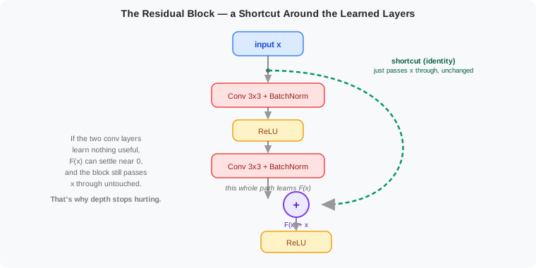
Instead of forcing layers to learn everything from scratch, the block learns a change to the input.
This is the key idea behind ResNet.
Why does this help?
If extra layers are useful, the model can use them.
If they are not useful, the model can pass information through the skip connection more easily.
Memory trick: A residual connection is like a shortcut road. The signal can go through the full path, but it also has a direct route if needed.
8. Global average pooling: avoid huge dense layers
In VGG16, the first dense layer is very large because it receives:
7 × 7 × 512 = 25,088 numbers
Then it connects those numbers to 4,096 neurons.
That creates more than 102 million parameters.
Modern CNNs often avoid this by using global average pooling.
Instead of flattening all values, global average pooling takes the average of each channel.
Example:
7 × 7 × 512 feature maps
→ average each 7 × 7 map
→ 512 numbers
So the classifier receives 512 numbers instead of 25,088.
This greatly reduces parameters.
Simple comparison:
| Method | Output to classifier |
|---|---|
| Flatten | 7 × 7 × 512 = 25,088 numbers |
| Global average pooling | 512 numbers |
Memory trick: Flatten keeps every location. Global average pooling summarizes each feature map into one score.
A related trick: 1x1 bottleneck convolutions
Global average pooling saves parameters at the very end of a network. A 1x1 convolution saves parameters throughout a deep network, using a different trick.
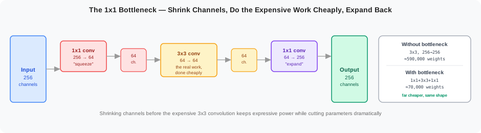
A 1x1 kernel doesn’t look at any neighboring pixels — its receptive field is a single position. At every position, it just mixes the channels together into a new, smaller (or larger) set of channels. That gives a cheap way to shrink the channel count right before an expensive 3x3 convolution, then expand it back afterward:
1x1 conv: squeeze 256 channels down to 64   (cheap)
3x3 conv: do the expensive work on just 64  (cheap, because fewer channels)
1x1 conv: expand 64 channels back to 256    (cheap)
The saving is large. A plain 3x3 convolution from 256 to 256 channels costs:
256 x (3x3x256) + 256 = 590,080 parameters
The bottleneck version — 1x1 (256→64), 3x3 (64→64), 1x1 (64→256) — costs:
16,448 + 36,928 + 16,640 = 70,016 parameters
Roughly eight times fewer parameters, for the same 256-channel output shape. This is one of the main tricks that let architectures deeper than VGG16 avoid VGG16’s biggest cost: enormous parameter counts.
bottleneck = nn.Sequential(
    nn.Conv2d(256, 64, kernel_size=1), nn.BatchNorm2d(64), nn.ReLU(),
    nn.Conv2d(64, 64, kernel_size=3, padding=1), nn.BatchNorm2d(64), nn.ReLU(),
    nn.Conv2d(64, 256, kernel_size=1), nn.BatchNorm2d(256),
)
Memory trick: A 1x1 convolution is a tiny accountant standing at one pixel, re-summarizing that pixel’s channels into a cheaper set of numbers — no neighbors involved.
9. Transfer learning: reuse a trained CNN
Training a large CNN from scratch needs many images and lots of compute.
But many CNNs have already been trained on huge datasets like ImageNet.
Transfer learning means reusing one of those trained models.
The idea:
Use pretrained CNN feature extractor
→ replace the final classifier
→ train for your own classes
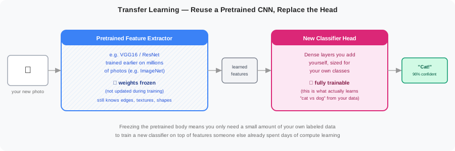
For example, a pretrained model already knows many visual basics:
- edges
- textures
- shapes
- object parts
You can reuse that knowledge for a new task.
Example tasks:
| Pretrained model learned | Your new task |
|---|---|
| General image patterns | Cat vs dog classifier |
| Object parts and textures | Medical image classifier |
| Shapes and colors | Product image classifier |
Transfer learning is useful when your dataset is not huge.
10. Freezing layers: train only part of the model
When using transfer learning, we often freeze earlier layers.
Freeze means:
Do not update these weights during training
Why freeze early layers?
Early CNN layers learn general patterns like edges and corners. Those are useful for many image tasks.
So we can keep them and train only the final classifier.
Simple flow:
Pretrained CNN feature extractor → frozen
New classifier head              → trainable
Later, if needed, we can unfreeze some deeper layers and fine-tune them gently.
11. Backpropagation in CNNs: how filters learn
Now let us connect CNN architecture with CNN learning.
A CNN has two main phases during training:
1. Forward pass  → make a prediction
2. Backward pass → learn from the mistake
The whole goal is simple:
Change the CNN’s weights and biases so the next prediction becomes better.
Where are the learnable parameters in a CNN?
Not every CNN layer learns weights.
| Layer | Has learnable weights and biases? | What happens during training? |
|---|---|---|
| Convolution layer | Yes | Kernels/filters are updated |
| Pooling layer | No | Only passes information forward/backward |
| Flatten layer | No | Only reshapes data |
| Dense layer | Yes | Dense weights and biases are updated |
So when we say CNN training, we mainly mean:
update convolution filters
update convolution biases
update dense layer weights
update dense layer biases
Step 1: forward pass
The forward pass means the image travels from input to output.
image
→ convolution
→ ReLU
→ pooling
→ flatten
→ dense layers
→ prediction
Example:
input image: cat
model output: 70% dog, 30% cat
The model made a wrong prediction.
Now it needs to learn from that mistake.
What happens inside convolution during the forward pass?
A convolution layer contains kernels, also called filters.
A filter is a small grid of weights.
Example:
3 × 3 filter = 9 weights for one input channel
For an RGB image, the filter looks across 3 channels:
3 × 3 × 3 = 27 weights
The filter slides over the image like a small window.
At each position:
image patch × filter weights + bias = one output number
After the filter scans the image, it creates a feature map.
one filter → one feature map
many filters → many feature maps
Each filter has its own weights and one bias. These are learnable parameters.
What happens inside pooling and flatten?
Pooling does not learn weights.
Max pooling only keeps the strongest value from a small region.
[5, 10]
[15, 16]
Max pooling keeps:
16
Flatten also does not learn weights.
It only reshapes feature maps into one long vector.
many 2D feature maps → one 1D vector
So pooling and flatten help data move through the CNN, but they do not store learned knowledge.
Step 2: calculate the loss
After the forward pass, the model has a prediction.
The true answer is also known during training.
prediction: 70% dog
true label: cat
The loss function measures the mistake.
For classification, a common loss is cross-entropy loss.
Simple meaning:
small loss → prediction is close to correct
large loss → prediction is far from correct
The loss gives backpropagation a target:
Reduce this mistake next time.
Step 3: backward pass
The backward pass starts from the loss and moves backward through the network.
loss
→ dense layers
→ flatten
→ pooling
→ ReLU
→ convolution filters
Backpropagation asks one repeated question:
How much did this weight contribute to the mistake?
The answer is called a gradient.
A gradient tells the optimizer how to change a weight.
gradient says weight is too high  → decrease it a little
gradient says weight is too low   → increase it a little
Then the optimizer updates the weight.
new weight = old weight - learning rate × gradient
The learning rate controls how big each update step is.
Backpropagation through dense layers
Dense layers work like the neural network layers from earlier parts.
Each connection has a weight.
Each neuron has a bias.
During backpropagation, the CNN updates:
dense weights
dense biases
This helps the final classifier combine image clues better.
Example:
ear clue + fur clue + eye clue → cat score
snout clue + tail clue         → dog score
If those combinations caused a wrong prediction, backpropagation adjusts the dense layer weights.
Backpropagation through flatten
Flatten has no weights.
So there is nothing to update.
During the backward pass, flatten simply reshapes the gradient back to the earlier feature map shape.
forward:  feature maps → long vector
backward: long vector gradient → feature map gradient
Backpropagation through max pooling
Max pooling also has no weights.
But it must still pass the gradient backward.
During the forward pass, max pooling remembers which value was the maximum.
Example:
[5, 10]
[15, 16]
The winner was 16.
During the backward pass, the gradient goes back only to that winning position.
[0, 0]
[0, gradient]
The other positions receive 0 because they were not selected by max pooling.
Backpropagation through ReLU
ReLU also has no weights.
But it controls whether gradients can pass backward.
Forward pass:
positive value → keep it
negative value → turn it into 0
Backward pass:
positive path → gradient passes through
zero path     → gradient is blocked
So ReLU behaves like a gate.
Backpropagation through convolution filters
Now the gradient reaches the convolution layer.
This is where CNN-specific learning happens.
A convolution filter was used many times while sliding across the image.
The same filter looked at many different patches.
So during backpropagation, the CNN collects learning signals from all those positions.
Then it updates the filter weights.
Simple idea:
filter detected useful pattern    → strengthen useful weights
filter caused wrong/confusing clue → adjust weights to reduce mistake
Each filter weight receives its own gradient.
Each filter bias also receives a gradient.
Then the optimizer updates them:
old filter
→ gradients from many image patches
→ updated filter
→ better pattern detector
This is how a random filter slowly becomes an edge detector, texture detector, curve detector, or object-part detector.
Full CNN learning flow
Forward pass:
image
→ filters create feature maps
→ ReLU keeps useful positive signals
→ pooling keeps strongest signals
→ flatten creates a vector
→ dense layers make prediction
→ loss measures mistake
Backward pass:
loss sends correction backward
→ dense weights are updated
→ flatten reshapes gradients
→ pooling sends gradient to winning locations
→ ReLU blocks gradients where values were zero
→ convolution filters and biases are updated
Tiny PyTorch gradient check
This small example shows that convolution filters receive gradients.
import torch
import torch.nn as nn

conv = nn.Conv2d(3, 4, kernel_size=3, padding=1)
image = torch.randn(1, 3, 32, 32)
target = torch.randn(1, 4, 32, 32)

output = conv(image)
loss = ((output - target) ** 2).mean()
loss.backward()

print(conv.weight.grad.shape)  # torch.Size([4, 3, 3, 3])
print(conv.bias.grad.shape)    # torch.Size([4])
The gradient shape matches the filter shape:
4 filters, 3 input channels, 3 × 3 kernel
That means PyTorch calculated one gradient for every learnable filter weight.
Final beginner-friendly summary
CNN learning means:
make prediction
→ measure mistake
→ send mistake backward
→ update filters and dense weights
→ try again
The key idea is:
Backpropagation does not hand-code filters. It slowly adjusts filter weights so useful visual patterns become easier to detect.
Memory trick: Forward pass asks, “What do I see?” Backward pass asks, “How should my filters change so I make fewer mistakes next time?”
12. A modern CNN block
A beginner CNN block might look like this:
Conv → ReLU → Pool
A more modern block may look like this:
Conv → BatchNorm → ReLU → Conv → BatchNorm → ReLU → skip connection
Then pooling or downsampling may reduce the image size.
So advanced CNNs are not completely new ideas. They are the same foundation with better training support.
| Basic idea | Advanced improvement |
|---|---|
| Convolution | More layers and better blocks |
| ReLU | Often still used after normalization |
| Pooling | Sometimes replaced by strided convolution |
| Dense classifier | Often reduced with global average pooling |
| Training from scratch | Often replaced with transfer learning |
13. Small advanced CNN example in PyTorch
Here is a small example that adds batch normalization, dropout, and global average pooling.
import torch
import torch.nn as nn

class BetterCNN(nn.Module):
    def __init__(self):
        super().__init__()

        self.features = nn.Sequential(
            nn.Conv2d(3, 32, kernel_size=3, padding=1),
            nn.BatchNorm2d(32),
            nn.ReLU(),
            nn.MaxPool2d(2),

            nn.Conv2d(32, 64, kernel_size=3, padding=1),
            nn.BatchNorm2d(64),
            nn.ReLU(),
            nn.MaxPool2d(2),
        )

        self.classifier = nn.Sequential(
            nn.AdaptiveAvgPool2d((1, 1)),
            nn.Flatten(),
            nn.Dropout(0.3),
            nn.Linear(64, 2)
        )

    def forward(self, x):
        x = self.features(x)
        x = self.classifier(x)
        return x

model = BetterCNN()
image = torch.randn(1, 3, 32, 32)
output = model(image)
print(output.shape)  # torch.Size([1, 2])
Flow:
Image
→ Conv + BatchNorm + ReLU
→ Pool
→ Conv + BatchNorm + ReLU
→ Pool
→ Global average pooling
→ Dropout
→ Final class scores
14. Final mental model
Advanced CNNs are not separate from basic CNNs.
They are basic CNNs plus tools that make training better.
| Concept | Simple meaning |
|---|---|
| Data augmentation | Show the model varied versions of images |
| Dropout | Randomly hide signals during training to reduce memorization |
| Batch normalization | Keep values stable between layers |
| Residual connection | Add a shortcut so deep networks train better |
| Global average pooling | Summarize each feature map instead of flattening everything |
| 1x1 bottleneck convolution | Squeeze channels down, do the expensive work cheaply, expand back |
| CNN backpropagation | Send error signals backward to update filters, feature maps, ReLU gates, and pooling winners |
| Transfer learning | Reuse a CNN trained on a large dataset |
| Freezing | Keep some pretrained weights unchanged |
The full journey is:
Basic CNN
→ handles images better than fully connected networks
→ deeper CNN
→ needs stable training and less overfitting
→ advanced CNN tools
→ better real-world performance
Previous: Part 9: Convolutional Neural Networks (CNNs)
Next: Part 11: CNN Training Pipeline, Transfer Learning, and Visualization