
Deep Learning for Generative AI — Part 10: Self-Attention in Code with NumPy
Deep Learning for Generative AI — Part 10: Self-Attention in Code with NumPy
In Part 9 we worked through self-attention by hand. Now we’ll let the computer do it.
We’ll build self-attention in about 15 lines of Python using NumPy, a library for working with tables of numbers (matrices). We run one step at a time, print the result, and explain what it means in plain words.
You don’t need anything installed. Copy the code into Google Colab (free, runs in your browser), or into any Python where numpy is available, and you’ll get exactly the same numbers.
1. Our example
A 4-word sentence:
"I drink hot coffee"
| Symbol | Meaning | Our value |
|---|---|---|
| N | Number of words | 4 |
| D1 | Length of each word’s starting vector | 3 |
| D2 | Length of each word’s rich vector (the size we want) | 5 |
So we start with 4 short vectors (3 numbers each) and want to end with 4 richer vectors (5 numbers each).
2. Step 0: import NumPy
import numpy as np
np.set_printoptions(precision=2, suppress=True)   # print numbers with 2 decimals

words = ["I", "drink", "hot", "coffee"]
N, D1, D2 = 4, 3, 5
rng = np.random.default_rng(16)   # a random number generator with a fixed "seed"
What’s a seed? Random numbers from a computer are really a very long, fixed list. The seed picks where in the list to start. Using the same seed (16) means you get exactly the same “random” numbers as this page.
3. Step 1: the input matrix X
In a real model, X would hold the word embeddings (Part 1). Here we just make up random numbers between 0 and 1:
X = rng.uniform(0, 1, size=(N, D1))
print("X shape:", X.shape)
print(X)
X shape: (4, 3)
[[0.57 0.43 0.09]     ← I
 [0.35 0.62 0.02]     ← drink
 [0.87 0.85 0.04]     ← hot
 [0.8  0.18 0.7 ]]    ← coffee
In plain words: a table with one row per word, 4 rows and 3 columns. These are the plain, “starting” descriptions of each word. They don’t know anything about the other words yet.
uniform(0, 1) just means “any number between 0 and 1 is equally likely”, like spinning a fair dial.
4. Step 2: the three weight matrices
Next we need W_Q, W_K and W_V, the three matrices that create queries, keys and values.
W_Q = rng.uniform(-2, 2, size=(D1, D2))
W_K = rng.uniform(-2, 2, size=(D1, D2))
W_V = rng.uniform(-2, 2, size=(D1, D2))
print("W_Q shape:", W_Q.shape)
print(W_Q)
W_Q shape: (3, 5)
[[-1.38  0.77  1.83  1.94  0.65]
 [-1.35 -0.42 -0.89  1.82 -0.8 ]
 [ 0.24 -0.37 -1.45 -0.46  1.08]]
Important: in a real Transformer these are not random. They are learned during training. We fill them with random numbers here to show one snapshot, like a model that hasn’t started learning yet.
Why size 3 × 5? It has to “fit” X. A 4 × 3 table can only be multiplied by a 3 × something table: the inner numbers must match. The 5 is our chosen D2, so the result will have 5 columns.
X      ×   W_Q    =   Q
(4×3)      (3×5)      (4×5)
   └── must match ─┘
5. Step 3: get Q, K and V
Three multiplications. In NumPy, @ means matrix multiplication:
Q = X @ W_Q     # queries: what each word is looking for
K = X @ W_K     # keys:    what each word can offer
V = X @ W_V     # values:  what each word actually knows
print("Q shape:", Q.shape)
print(Q)
Q shape: (4, 5)
[[-1.34  0.22  0.52  1.84  0.13]     ← query of "I"
 [-1.31 -0.    0.06  1.8  -0.25]     ← query of "drink"
 [-2.35  0.29  0.78  3.23 -0.07]     ← query of "hot"
 [-1.19  0.28  0.3   1.57  1.13]]    ← query of "coffee"
K (4, 5)                                  V (4, 5)
[[ 0.26  1.1  -0.37 -0.19  0.99]  I       [[ 0.36 -0.33  1.24 -0.77  0.98]
 [ 0.35  1.04 -0.75  0.58  1.2 ]  drink    [ 0.02 -0.86  1.44 -0.11  0.66]
 [ 0.36  1.74 -0.89  0.12  1.98]  hot      [ 0.36 -0.95  2.22 -0.95  1.61]
 [ 0.97  2.08  0.34 -1.37 -0.22]] coffee   [ 1.29  0.95  1.3  -1.82  0.94]]
In plain words: each table has 4 rows (one per word) and 5 columns (D2). So every word now has its own query, key and value, each 5 numbers long.
Notice: one line of code handles all 4 words at once. No loop, no waiting for the previous word. That’s why Transformers are fast.
6. Step 4: match every query with every key
How much should each word listen to each other word? Compare its query with every word’s key:
scores = Q @ K.T        # K.T means "K transposed": rows turned into columns
print("scores shape:", scores.shape)
print(scores)
scores shape: (4, 4)
          I      drink   hot    coffee
I      [[-0.52   0.59  -0.11  -3.21]
drink   [-0.95   0.24  -0.81  -3.67]
hot     [-1.25   0.7   -0.79  -5.81]
coffee  [ 0.7    1.91   2.2   -2.87]]
Why 4 × 4? Every word (row) gets a score with every word (column), including itself. 4 words × 4 words = 16 scores.
What is a score? A score is a dot product: multiply the two lists of numbers position by position, then add everything up. Two lists that “agree” (big numbers in the same places, same signs) give a big total. Lists that disagree give a small or negative total.
For example, coffee vs hot = 2.2, the biggest in its row. So coffee’s query best matches hot’s key.
What does a negative score mean? Just “a poor match”. It doesn’t mean “hate”. Softmax will turn it into a small weight in the next step.
7. Step 5: turn scores into weights (scale + softmax)
We want weights that are between 0 and 1 and add up to 1 in every row, like slicing a pie. Two small steps:
scaled = scores / np.sqrt(D2)           # 1) calm the numbers down

def softmax(z):                         # 2) turn each row into a "pie"
    e = np.exp(z)
    return e / e.sum(axis=1, keepdims=True)

A = softmax(scaled)
print("A shape:", A.shape)
print(A)
print("row sums:", A.sum(axis=1))
A shape: (4, 4)
          I     drink  hot   coffee
I      [[0.24  0.4   0.29  0.07]
drink   [0.25  0.42  0.26  0.07]
hot     [0.21  0.5   0.26  0.03]
coffee  [0.21  0.35  0.4   0.04]]
row sums: [1. 1. 1. 1.]
Why divide by √D2? With long vectors, dot products can become huge, and softmax would then give one word nearly all the attention. Dividing by √D2 (here √5 ≈ 2.24) keeps the numbers in a sensible range. Think of it as turning the volume down before comparing.
What does softmax do, in simple terms?
np.exp(z)turns every number into a positive number. Bigger stays bigger, and negatives become small positives.- Divide each by the row total, so each row adds up to 1.
A tiny example with three scores:
scores:        -0.5     0.2     0.9
exp:            0.61    1.22    2.46      (total = 4.29)
÷ total:        0.14    0.28    0.57      ← adds up to 1, biggest score gets the biggest slice
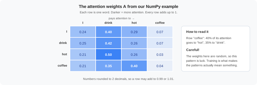
Reading the result: “coffee” puts 40% of its attention on “hot” and 35% on “drink”. Almost nobody pays attention to “coffee” itself.
Be careful: our weight matrices are random, so this nice-looking pattern is luck. In a trained model, W_Q and W_K are tuned so that patterns like “coffee → hot” appear because they’re actually useful.
8. Step 6: blend the values into rich vectors
Last step. Each word’s new vector is a weighted blend of all the values, using its row of A as the recipe:
Z = A @ V
print("Z shape:", Z.shape)
print(Z)
Z shape: (4, 5)
[[ 0.29 -0.63  1.61 -0.64  1.03]     ← new "I"
 [ 0.28 -0.62  1.59 -0.62  1.01]     ← new "drink"
 [ 0.21 -0.72  1.6  -0.51  0.98]     ← new "hot"
 [ 0.28 -0.71  1.71 -0.65  1.12]]    ← new "coffee"
Let’s check the first number for “coffee” ourselves. Its recipe (row of A) is 0.21 of I, 0.35 of drink, 0.40 of hot and 0.04 of coffee. Take the first number of each word’s value:
0.21 × 0.36  +  0.35 × 0.02  +  0.40 × 0.36  +  0.04 × 1.29
=  0.076     +  0.007       +  0.144       +  0.052
≈  0.28  ✓
Like a smoothie recipe: A says how much of each fruit (value) goes in, and Z is the smoothie. Every word gets its own recipe, so every word gets its own smoothie.
We did it: we turned a 4 × 3 table of plain word vectors into a 4 × 5 table of richer vectors, where each word now carries information from the whole sentence.
9. The whole thing in one block
Here is everything together. Paste it into Colab and run it:
import numpy as np
np.set_printoptions(precision=2, suppress=True)

N, D1, D2 = 4, 3, 5                       # 4 words, start size 3, target size 5
rng = np.random.default_rng(16)

X   = rng.uniform(0, 1, size=(N, D1))     # starting word vectors
W_Q = rng.uniform(-2, 2, size=(D1, D2))   # learned in real models
W_K = rng.uniform(-2, 2, size=(D1, D2))
W_V = rng.uniform(-2, 2, size=(D1, D2))

Q, K, V = X @ W_Q, X @ W_K, X @ W_V       # queries, keys, values

scores = Q @ K.T / np.sqrt(D2)            # how well each query matches each key
A = np.exp(scores) / np.exp(scores).sum(axis=1, keepdims=True)   # softmax
Z = A @ V                                 # blend the values

print(Z)                                  # 4 rich vectors, 5 numbers each
That is self-attention. The line Z = A @ V with A = softmax(Q Kᵀ / √D2) is exactly the formula from Part 9:
Z = softmax( Q Kᵀ / √D2 ) × V
10. Where does training come in?
Nothing above “learned” anything. We used random W_Q, W_K and W_V. In a real model:
start:   W_Q, W_K, W_V are random            → attention is messy, results are poor
train:   show the model lots of examples, and nudge W_Q, W_K, W_V
         a tiny bit after each mistake
end:     W_Q, W_K, W_V are well tuned         → queries and keys match in useful ways
                                             → attention weights make sense
                                             → rich vectors Z are genuinely useful
The training process only changes these three matrices (plus the other layers from Part 8). Get them right, and everything else falls into place.
The same code works for self-attention in the decoder too. The only extra step there is the mask from Part 8: set the scores for future words to a huge negative number before softmax, so their weight becomes 0.
11. Summary
| Step | Code | Shape | Plain meaning |
|---|---|---|---|
| Input | X |
4 × 3 | One starting vector per word |
| Weights | W_Q, W_K, W_V |
3 × 5 | Learned in training (random here) |
| Q, K, V | X @ W_Q … |
4 × 5 | Each word’s question, offer, knowledge |
| Scores | Q @ K.T |
4 × 4 | How well every query matches every key |
| Weights | softmax(scores / √D2) |
4 × 4 | Each row is a pie that adds up to 1 |
| Output | A @ V |
4 × 5 | A custom blend of values for each word |
- Self-attention is a handful of matrix multiplications, and NumPy does each in one line.
- Every word is handled at the same time.
- Random weights give random-looking attention. Training is what makes it meaningful.
Next up: most modern models keep only half of the Transformer. Find out which half and why in Part 11: Transformer Variants — Encoder-Only, Decoder-Only, Encoder-Decoder.