
Deep Learning for Generative AI — Part 2: Encoder-Decoder Architecture
Deep Learning for Generative AI — Part 2: Encoder-Decoder Architecture
In Part 1 we turned words into numbers (embeddings). Now we need a network that can read a whole sentence and produce a different sentence — for example, translating English to French or summarising a paragraph.
The architecture that does this is called encoder-decoder, also known as sequence-to-sequence (seq2seq). The important thing to know upfront: the encoder and decoder are two separate neural networks, each with its own weights. They are trained together but they do different jobs.
1. The foundation: translation is done by neural networks
Our goal in this article is to translate a sentence — say, English to French:
"I love cats" → "J'aime les chats"
The machine that does this is built from neural networks. So before we look at the architecture, let’s understand what a neural network does in the context of translation.
A neural network only works with numbers
A neural network cannot read words. It takes numbers in and produces numbers out. So the entire translation pipeline is about numbers:
"I love cats"                                    "J'aime les chats"
      ↓                                                  ↑
convert words to numbers                    convert numbers back to words
      ↓                                                  ↑
[0.12, -0.45, ...]  →  [neural networks]  →  [0.87, 0.03, ...]
- Going in: each word becomes a vector of numbers (the embeddings from Part 1).
- Inside: the networks transform these numbers step by step.
- Coming out: the final numbers are converted back into words (by picking the most likely word from the vocabulary).
How does the network transform numbers? Weights.
Inside the network are weights — grids of numbers (matrices). Every transformation is a matrix multiplication: the input numbers get multiplied by the weights to produce output numbers.
Here is a tiny example. Say the word vector for “I” is [0.8, 0.2] and the network has this weight matrix:
       input for "I"    weights           output
       [0.8]            [[0.6, 0.1],      [?]
       [0.2]             [0.2, 0.7]]      [?]

output[0] = 0.6 × 0.8 + 0.1 × 0.2 = 0.50
output[1] = 0.2 × 0.8 + 0.7 × 0.2 = 0.30

output = [0.50, 0.30]
The weights decide what the network pays attention to in the word vector. Different weights would produce a completely different output from the same word.
Where do the weights come from? Training.
The weights start as random numbers — at that point the network produces garbage translations. Then we train it:
- Show it an example: Feed in “I love cats” and let the network produce a translation attempt — maybe “Le chien mange” (garbage at first).
- Measure the error: Compare the attempt with the correct answer “J’aime les chats.” The difference is called the loss.
- Adjust the weights: A process called backpropagation figures out which weights caused the error and nudges each one slightly in the direction that reduces it.
- Repeat with millions of sentence pairs. Gradually the weights shift from random values to values that produce correct translations.
                  ┌──────────────────────────────────────────────┐
                  │  Feed in "I love cats" → get attempt          │
  Training loop:  │  Compare with "J'aime les chats" → loss       │
                  │  Backpropagation → nudge all weights slightly │
                  │  Repeat with the next sentence pair           │
                  └──────────────────────────────────────────────┘
Nobody programs the translation rules by hand. The network discovers them by seeing millions of translated sentence pairs and slowly adjusting its weights.
What you need before training: parallel examples
All of this depends on having a dataset of input–output pairs. For translation, each example is one sentence in the source language paired with its translation in the target language:
Input:  "I love cats"
Output: "J'aime les chats"
The same idea works for other tasks. An English-to-Python pair might look like:
Input:  "Python program to print Hello World"
Output: print("Hello World")
The model learns by comparing its attempt with the correct output. Higher-quality, larger datasets give better translations — the model can only learn patterns that appear in the data it sees.
Keep this in mind for the rest of the article
Everything that follows builds on these three facts:
- The translator is made of neural networks that only handle numbers.
- The transformations happen through weight matrices (like
W_h,W_x, andbyou will see later). - Those weights are learned from training data, not written by a person.
2. The problem: variable-length input → variable-length output
Now that we know translation is done by neural networks, here is the first obstacle. The network from section 1 takes a fixed-size input and gives a fixed-size output. But sentences come in all sizes:
Input:  "How are you?"          (3 words)
Output: "Comment allez-vous ?"  (3 words, but could be 2 or 5)
We need a model that can handle any length on both sides. The solution is the encoder-decoder architecture.
3. The big idea: two networks working together
The encoder-decoder uses two separate neural networks that work as a team:
┌─────────────────────────┐         ┌─────────────────────────┐
│    ENCODER (network 1)  │         │    DECODER (network 2)  │
│                         │         │                         │
│  Has its own weights    │ context │  Has its own weights    │
│  Job: read the input    │ vector  │  Job: generate output   │
│  sentence and compress  │────────→│  sentence, one word at  │
│  it into a single vector│         │  a time                 │
└─────────────────────────┘         └─────────────────────────┘
- Network 1 (encoder): reads the input sentence and compresses it into a single vector.
- Network 2 (decoder): takes that vector and generates the output sentence, one word at a time.
They have separate weight matrices — the encoder has its own W_h and W_x, and the decoder has its own different W_h and W_x. But they are trained together as one system: the loss from the decoder’s output flows back through both networks, so both sets of weights are updated at the same time.
Analogy: the interpreter
Imagine an interpreter at the United Nations. A delegate speaks a full sentence in English, and the interpreter must repeat it in French.
The interpreter works in two phases:
-
Listening phase (encoder): The interpreter listens to the entire English sentence from start to finish. While listening, they do not speak — they just build up an understanding of what was said. By the end of the sentence, the interpreter holds the full meaning in their head.
-
Speaking phase (decoder): Now the interpreter opens their mouth and produces the French translation, one word at a time. They are no longer listening to the original English — they are working entirely from the understanding they built during the listening phase.
The key point is what happens between these two phases. After listening and before speaking, the interpreter holds a mental summary — they know what the sentence means, even though they have not started translating yet. In the neural network, this mental summary is called the context vector. It is a list of numbers (e.g. 256 or 512 numbers) that represents the meaning of the entire input sentence.
English sentence → [interpreter listens] → mental summary → [interpreter speaks] → French sentence
English sentence → [encoder processes]   → context vector → [decoder generates]  → French sentence
The context vector is the only connection between the encoder and the decoder. The decoder never sees the original English words — it only gets this one vector. So the context vector must contain everything the decoder needs to produce the correct output.
That is the big picture. Now let’s follow the pipeline step by step, starting with how words get into the encoder in the first place.
4. First step: every word becomes a vector
Before the encoder can process anything, each word must be turned into a vector of numbers. This is the embedding step we covered in Part 1.
Here is what happens to the sentence “I love cats.” We will use the same tiny six-word English vocabulary throughout this article:
Step 1 — Tokenise:  split the sentence into tokens
  "I love cats"  →  ["I", "love", "cats"]

Step 2 — Convert each token to its ID using the tokenizer's vocabulary

  Token:   I   love   cats   dogs   you   the
  ID:      0     1      2      3     4     5

  ["I", "love", "cats"]  →  [0, 1, 2]

Step 3 — Use each ID as a row number in the embedding matrix

  Row 0 ("I")    → [0.12, -0.45,  0.78]
  Row 1 ("love") → [0.91,  0.02, -0.64]
  Row 2 ("cats") → [0.34,  0.88,  0.21]
Where did IDs 0, 1, and 2 come from? Before training, the tokenizer builds this token → ID vocabulary mapping, or loads a vocabulary that was built earlier. Once assigned, the IDs stay fixed: every occurrence of "cats" becomes 2, and 2 always selects row 2. The ID itself contains no meaning—it is only an address, like a row number in a spreadsheet. The values stored at that address are what the model learns.
This walkthrough uses whole words to keep the architecture easy to see. Modern tokenizers often split text into subword tokens, but the mechanism is unchanged: each token has a fixed vocabulary ID, and that ID selects one embedding row. Real embedding rows also contain many more values, such as 256 instead of the 3 shown here.
So the sentence is now a sequence of vectors — one vector per word:
"I love cats"
      ↓
[ [0.12, -0.45, 0.78],    ← vector for "I"
  [0.91,  0.02, -0.64],   ← vector for "love"
  [0.34,  0.88,  0.21] ]  ← vector for "cats"
These embedding vectors are what the encoder actually receives. It never sees the raw words — it only sees numbers.
Where does the embedding matrix come from? It has one row for every entry in the tokenizer’s vocabulary. Its values can come from pre-trained embeddings (like Word2Vec or GloVe from Part 1), or they can start as random numbers and be trained along with the rest of the network. Training updates the values inside the rows so the vectors become more meaningful; it does not keep changing which token ID selects which row.
We now have a sequence of word vectors. The next step is to feed them to the first of our two networks: the encoder.
5. The encoder
The encoder’s job is to read the word vectors from section 4, one at a time, and build up a single summary of the whole sentence.
The problem: a normal network has no memory
Recall the neural network from section 1: numbers go in, math happens, numbers come out. Each input is processed independently — the network has no idea what it saw before.
Normal network:

  input 1 → [network] → output 1     (forgets everything)
  input 2 → [network] → output 2     (forgets everything)
  input 3 → [network] → output 3     (forgets everything)
That is a problem for sentences, because word order and history matter. “The dog bit the man” and “The man bit the dog” contain the same words — the only difference is the sequence. To understand a sentence, the network must remember what came before.
The solution: give the network a memory (this is the RNN)
How do we fix a network that forgets? Simple idea: whatever the network produced for the previous word, hand it back to the network along with the next word.
Compare the two side by side:
Normal network — each word processed alone:

  "I"    → [network] → result       (result is thrown away)
  "love" → [network] → result       (knows nothing about "I")
  "cats" → [network] → result       (knows nothing about "I love")


RNN — each word processed together with the previous result:

  "I"    + (blank memory)        → [network] → memory after "I"
                                                    │
                                     ┌──────────────┘
                                     ↓
  "love" + memory after "I"      → [network] → memory after "I love"
                                                    │
                                     ┌──────────────┘
                                     ↓
  "cats" + memory after "I love" → [network] → memory after "I love cats"
Notice what changed: the network now takes two inputs at every step instead of one:
- The new word (as a vector, from section 4)
- The memory from the previous step (what the network produced last time)
And it produces one output: an updated memory that now includes the new word.
Important: it is the same network with the same weights used at every step — not three different networks. The network is simply applied again and again, once per word, each time carrying its previous output forward.
Analogy: reading with a sticky note
Imagine you can only see one word at a time through a small window, but you have a sticky note:
- You see “I” — you write on the note: “someone is talking about themselves.”
- The window moves to “love” — you read your note, see the new word, and rewrite the note: “this person loves something.”
- The window moves to “cats” — you read the note, see the new word, and rewrite: “this person loves cats.”
You never saw the whole sentence at once — but by always combining the note (memory) with the current word, you ended up understanding the full sentence. The RNN does exactly this.
This is why it is called recurrent — “recurrent” means “happening repeatedly.” The same operation repeats for every word, and the output of one step feeds back in as the input of the next.
Where exactly does this loop live inside the network?
A neural network has three parts: an input layer, one or more middle (hidden) layers, and an output layer. The loop is not at the output layer — it happens at the middle layer.
Here is a normal feed-forward network first:
Normal network (no memory):

   input layer      middle layer      output layer
   ┌─────────┐      ┌───────────┐     ┌──────────┐
   │  word   │ ───→ │  neurons  │ ──→ │  result  │
   │ vector  │      │ (compute) │     │          │
   └─────────┘      └───────────┘     └──────────┘

   Data flows straight through, left to right. Nothing is kept.
And here is the RNN — one added connection makes all the difference:
RNN (with memory):

   input layer      middle layer      output layer
   ┌─────────┐      ┌───────────┐     ┌──────────┐
   │  word   │ ───→ │  neurons  │ ──→ │  result  │
   │ vector  │      │ (compute) │     │(optional)│
   └─────────┘      └─────┬─────┘     └──────────┘
                      ↑    │
                      │    │  the middle layer's values
                      └────┘  loop back into itself
                              at the next time step
The values sitting in the middle layer after processing a word — those are the hidden state. At the next time step, they are fed back into the same middle layer along with the new word.
Unrolled over time, it looks like this:
              "I"              "love"            "cats"
               │                 │                 │
               ↓                 ↓                 ↓
          ┌─────────┐       ┌─────────┐       ┌─────────┐
  h0 ───→ │ middle  │ ─h1─→ │ middle  │ ─h2─→ │ middle  │ ─h3─→ context
 (zeros)  │  layer  │       │  layer  │       │  layer  │       vector
          └─────────┘       └─────────┘       └─────────┘
          (same layer, same weights, applied 3 times)
Two things to notice:
- The hidden state h is the middle layer’s activations — not a separate storage box. “Passing the hidden state forward” literally means: take the middle layer’s numbers from this step and feed them into the middle layer at the next step.
- The output layer is optional for the encoder. The encoder does not need to produce a word at every step — we only care about its final hidden state (the context vector). The decoder, on the other hand, does use its output layer at every step to predict the next word.
What about stacked layers? If the encoder has 3 stacked layers (as shown later in this section), each layer has its own loop and its own hidden state. Layer 1’s hidden state feeds back into layer 1, layer 2’s into layer 2, and so on.
Stacked RNN — every layer has its own loop:

   word vector
        ↓
   ┌─────────┐ ←──┐
   │ layer 1 │────┘   h¹ loops back into layer 1
   └────┬────┘
        ↓
   ┌─────────┐ ←──┐
   │ layer 2 │────┘   h² loops back into layer 2
   └────┬────┘
        ↓
   ┌─────────┐ ←──┐
   │ layer 3 │────┘   h³ loops back into layer 3
   └────┬────┘
        ↓
     output
But wait — for images, the whole image goes in at once. Why not the whole sentence?
If you have seen image networks (like CNNs), you know the entire image is fed into the first layer in one go, and there is one forward pass:
Image network — ONE forward pass, whole input at once:

  entire image (e.g. 224×224 pixels, all at once)
        ↓
   [layer 1] → [layer 2] → [layer 3] → "cat"

  Run once. Done.
An RNN is different: the network runs once per word — a 3-word sentence means 3 forward passes through the same network:
RNN — THREE forward passes, one word each:

  Pass 1:  "I"    + h0 → [network] → h1
  Pass 2:  "love" + h1 → [network] → h2
  Pass 3:  "cats" + h2 → [network] → h3

  Run 3 times. The hidden state carries information between runs.
Why the difference?
| Image | Sentence | |
|---|---|---|
| Size | Fixed (e.g. always 224×224 pixels) | Variable (3 words, 8 words, 50 words…) |
| Input strategy | Whole input in one pass | One word per pass, repeated |
| Memory between passes | Not needed — there is only one pass | The hidden state connects the passes |
An image always has the same number of pixels, so you can build a network whose input layer exactly fits it. A sentence has no fixed size — you cannot build an input layer that fits “any number of words.” The RNN’s trick is to keep the network small (one word at a time) and run it repeatedly, using the hidden state to accumulate meaning across the runs.
In short: an image network is one big bite; an RNN is many small bites with a memory of what it has chewed so far.
Fun fact: the Transformer architecture (coming in later parts) actually does take the whole sentence at once, more like an image network — that is one of the reasons it replaced RNNs. But it needs special tricks (positional encoding, attention) to handle variable lengths and word order.
That memory has a name: the hidden state
The memory that gets passed from step to step is called the hidden state. Concretely, it is just a list of numbers (e.g. 256 numbers):
- It is called hidden because it is internal to the network — it is not the input and not the final output; it lives “hidden” in the middle.
- It is called a state because it represents the network’s current state of understanding — everything it has absorbed from the sentence so far.
It starts as all zeros — the encoder knows nothing yet. Every time it reads a new word, it updates this memory.
Think of it like taking notes while listening to someone speak:
- Before they start → your notepad is blank (hidden state = all zeros)
- After hearing the first word → you jot down a rough note (hidden state h1)
- After hearing the second word → you update your notes with the new information (hidden state h2)
- After the last word → your notes now summarise everything that was said (final hidden state = context vector)
The key idea: the hidden state always has the same size (e.g. always 256 numbers), no matter how many words you have read. It is a fixed-size notepad that keeps getting rewritten.
Note: In practice the encoder is usually an LSTM or GRU rather than a plain RNN. These are improved versions of the RNN that are better at remembering things over long sentences, but the core idea — a hidden state updated word by word — is exactly the same.
Walking through “I love cats”
Let’s say our hidden state has 4 numbers (real models use 256–512, but 4 is easier to follow).
Before starting: the hidden state is zeros.
h0 = [0, 0, 0, 0] (encoder knows nothing)
Step 1 — Read “I”:
The encoder takes two inputs: the word vector for “I” and the current hidden state h0. It mixes them together (using learned weights) and produces a new hidden state:
Input:   word vector for "I" = [0.12, -0.45, 0.78, 0.33]
         previous state  h0  = [0, 0, 0, 0]

Output:  new state  h1 = [0.31, -0.12, 0.55, 0.08]
h1 now contains the encoder’s understanding after reading just “I” — it knows someone is the subject.
Step 2 — Read “love”:
Input:   word vector for "love" = [0.91, 0.02, -0.64, 0.17]
         previous state  h1     = [0.31, -0.12, 0.55, 0.08]

Output:  new state  h2 = [0.68, 0.24, -0.11, 0.42]
h2 now captures “I love” — the encoder knows someone loves something.
Step 3 — Read “cats”:
Input:   word vector for "cats" = [0.34, 0.88, 0.21, -0.55]
         previous state  h2     = [0.68, 0.24, -0.11, 0.42]

Output:  new state  h3 = [0.52, 0.71, 0.33, -0.19]
h3 now captures the meaning of the entire sentence “I love cats.” This final hidden state is the context vector.
context vector = h3 = [0.52, 0.71, 0.33, -0.19]
How does the encoder “mix” the word vector with the hidden state?
It is not simple vector addition. The encoder uses three operations: matrix multiplication, addition, and squashing. Here is the formula:
h_t = tanh(W_h × h_{t-1} + W_x × x_t + b)
That looks dense, so let’s break it into three clear sub-steps:
Sub-step 1:  Transform the memory      →  W_h × h_{t-1}      (matrix multiply)
Sub-step 2:  Transform the new word     →  W_x × x_t          (matrix multiply)
Sub-step 3:  Add them together + bias   →  result + b          (addition)
Sub-step 4:  Squash to [-1, +1]         →  tanh(result)        (activation)
The activation function runs at every step. The value saved as the new hidden state h_t is the result after tanh, so the memory passed to the next step is already squashed into the [-1, +1] range.
Why matrix multiplication and not just addition?
Plain addition would just pile numbers on top of each other — the encoder would have no control over which parts of the word or memory matter. Matrix multiplication is like a set of knobs and dials: each weight in the matrix controls how much one input number influences one output number. This lets the encoder learn things like “pay a lot of attention to verbs but less to articles.”
Worked example with real numbers
Let’s use tiny 2-dimensional vectors so you can follow every number. In a real model these would be 256 or 512 dimensions — the math is identical, just bigger.
Important: where does each number come from?
| Value | Where it comes from | In this example |
|---|---|---|
h0 (previous hidden state) |
The output of the previous step. At the very start of a sentence, it is initialised to all zeros. Here we use [0.5, -0.3] to show a mid-sentence step where the encoder already has some memory. |
[0.5, -0.3] |
x1 (word vector) |
Looked up from the embedding matrix (section 4). The word “I” has an index in the vocabulary, and that index picks a row from the embedding table. | [0.8, 0.2] |
W_h (weight matrix for memory) |
Initialised randomly before training, then learned by backpropagation. The network adjusts these numbers over thousands of training examples until they produce good translations. | [[0.1, 0.4], [0.3, 0.2]] |
W_x (weight matrix for word) |
Same as W_h — randomly initialised, then learned during training. | [[0.6, 0.1], [0.2, 0.7]] |
b (bias) |
Also learned during training. We set it to zero here to keep the example simple. | [0.0, 0.0] |
So: h0 comes from the previous step, x1 comes from the embedding table, and W_h, W_x, b are all learned parameters that the network discovers during training. Nobody chooses these numbers by hand — the training process finds values that work.
Given (made-up numbers for illustration):
Previous hidden state:  h0     = [0.5, -0.3]
New word vector:        x1     = [0.8,  0.2]    (the word "I")

Weight matrix for memory:  W_h = [[0.1, 0.4],
                                   [0.3, 0.2]]

Weight matrix for word:    W_x = [[0.6, 0.1],
                                   [0.2, 0.7]]

Bias:                      b   = [0.0, 0.0]     (zero for simplicity)
Sub-step 1 — Transform the memory (W_h × h0):
This is matrix-vector multiplication. Each output number is a dot product of one row of W_h with h0:
row 1:  0.1 × 0.5  +  0.4 × (-0.3)  =  0.05 + (-0.12)  =  -0.07
row 2:  0.3 × 0.5  +  0.2 × (-0.3)  =  0.15 + (-0.06)  =   0.09

W_h × h0 = [-0.07, 0.09]
Sub-step 2 — Transform the new word (W_x × x1):
row 1:  0.6 × 0.8  +  0.1 × 0.2  =  0.48 + 0.02  =  0.50
row 2:  0.2 × 0.8  +  0.7 × 0.2  =  0.16 + 0.14  =  0.30

W_x × x1 = [0.50, 0.30]
Sub-step 3 — Add them together (+ bias):
[-0.07, 0.09] + [0.50, 0.30] + [0.0, 0.0] = [0.43, 0.39]
This is the only step that uses plain addition — and it is adding two transformed vectors, not the raw inputs.
Sub-step 4 — Squash with tanh:
tanh pushes every number into the range [−1, +1]:
tanh(0.43) = 0.41
tanh(0.39) = 0.37

h1 = [0.41, 0.37]   ← the new hidden state
Summary of what happened:
h0 = [0.5, -0.3]    (old memory)
x1 = [0.8, 0.2]     (new word "I")
        ↓
   matrix multiply each with learned weights
        ↓
   add the two transformed results
        ↓
   squash with tanh
        ↓
h1 = [0.41, 0.37]   (updated memory)
The weight matrices decide how much of the old memory to keep and how much of the new word to absorb. During training, the network adjusts these weights so that the final hidden state captures the most useful information from the sentence.
Quick reference table
| Symbol | What it is | Plain English |
|---|---|---|
x_t |
The embedding vector of the current word | The new word the encoder is reading right now |
h_{t-1} |
The previous hidden state | The encoder’s memory from all previous words |
W_x |
A weight matrix for the word | Controls how the new word is transformed |
W_h |
A weight matrix for the memory | Controls how the old memory is transformed |
b |
A bias term | A small adjustment (like a default starting point) |
tanh |
An activation function | Squashes the result to stay between −1 and +1 |
h_t |
The new hidden state | The encoder’s updated memory after tanh; these post-activation values become the memory for the next step |
The weight matrices W_x and W_h are learned during training. The network figures out for itself how to best combine new words with existing memory.
Analogy: mixing paint
Think of each word vector as a new colour of paint. The hidden state is the colour in your bucket:
- Bucket starts empty (clear).
- Pour in “I” (blue) → bucket is now blue.
- Pour in “love” (red) → bucket is now purple (a mix of blue and red).
- Pour in “cats” (yellow) → bucket is now a brownish mix of all three.
The final colour represents the whole sentence. You cannot separate the individual colours out again — they are blended. This is both the strength (compact summary) and the weakness (you lose individual word detail) of this approach.
After the last word, the hidden state contains a compressed representation of the entire sentence. This is the context vector that gets passed to the decoder.
How many layers do the encoder and decoder have?
So far we showed a single-layer RNN — one set of weights processes the word vectors. But in practice, encoder-decoders stack multiple layers on top of each other. This is called a stacked or deep RNN.
Single layer (what we showed above)
word vectors:   x1 → x2 → x3
                 ↓     ↓     ↓
Layer 1:        h1 → h2 → h3  → context vector
One layer reads the words left to right and produces one hidden state per word.
Stacked layers (what real models use)
word vectors:    x1  →  x2  →  x3
                  ↓      ↓      ↓
Layer 1:        h1¹ → h2¹ → h3¹        (captures basic patterns)
                  ↓      ↓      ↓
Layer 2:        h1² → h2² → h3²        (captures deeper patterns)
                  ↓      ↓      ↓
Layer 3:        h1³ → h2³ → h3³        (captures even deeper patterns)
                                 ↓
                          context vector = h3³
Each layer takes the outputs of the layer below as its input. The bottom layer sees the raw word vectors. The next layer sees the hidden states from below, and learns higher-level patterns from them — like understanding phrase structure or sentence meaning rather than just individual words.
Typical numbers
| Model | Encoder layers | Decoder layers | Hidden size |
|---|---|---|---|
| Simple seq2seq (tutorial) | 1 | 1 | 256 |
| Google’s original NMT (2016) | 4 | 4 | 1,024 |
| Larger production models | 4–8 | 4–8 | 512–1,024 |
More layers = more capacity to learn complex patterns, but also slower to train and more likely to overfit on small datasets. The encoder and decoder usually have the same number of layers so the hidden states match in size when passing the context vector.
The decoder works the same way — if it has 3 layers, each decoder step runs through all 3 layers before predicting the next word.
6. The context vector
Let’s zoom in on the hand-off between the two networks. From the walkthrough in section 5, the encoder’s final hidden state was:
"I love cats" → context vector c = h3 = [0.52, 0.71, 0.33, -0.19]
This single vector (in real models 256 or 512 numbers) is the bridge between the encoder and decoder. It must summarise the entire input sentence, because it is the only thing the decoder receives.
This is both the power and the weakness of this design:
- Power: any input length gets compressed to the same fixed size, so the decoder always knows what to expect.
- Weakness: a 50-word sentence must squeeze into the same space as a 3-word sentence — information gets lost. (This is the paint-mixing problem from section 5, and it is the main motivation for attention in Part 3.)
7. The decoder
Now for the second network. The decoder is another RNN — it works with a hidden state just like the encoder, but its job is reversed: instead of reading words to build a summary, it starts from the summary (the context vector) and unfolds it into words, one at a time.
Initial state: context vector c

Step 1: Input <START> token → predict "J'"     → hidden state s1
Step 2: Input "J'"          → predict "aime"   → hidden state s2
Step 3: Input "aime"        → predict "les"    → hidden state s3
Step 4: Input "les"         → predict "chats"  → hidden state s4
Step 5: Input "chats"       → predict <END>    → stop
At each step the decoder:
- Takes the previous word (or
<START>at the beginning) - Updates its hidden state — same mixing operation as the encoder, but with the decoder’s own weights
- Predicts the next word using a softmax over the vocabulary
What is softmax? The decoder’s final layer produces one score for every word in the vocabulary (e.g. 30,000 scores). Softmax converts these scores into probabilities that add up to 1. The word with the highest probability is picked as the next output word:
Decoder scores  →  softmax  →  P("J'") = 0.72, P("Je") = 0.15, P("Le") = 0.04, ...
                                        ↓
                              pick "J'" (highest probability)
Training vs inference
The decoder behaves differently depending on whether it is being trained or being used. First, the two terms:
- Training: the model is learning. We have the correct translation (“J’aime les chats”) and we are adjusting the weights.
- Inference: the model is being used for real. There is no correct answer available — the model is on its own.
The difference is in what we feed into each decoder step as the “previous word.”
During inference: the model uses its own predictions
There is no other choice — we do not know the correct answer. Whatever the model predicted at step 1 becomes the input for step 2:
Step 1: <START>          → predicts "J'"
Step 2: "J'" (own guess) → predicts "aime"
Step 3: "aime"           → predicts "les"
...
The danger: if the model makes a mistake early, that mistake is fed into the next step, which can cause another mistake — errors compound:
Step 1: <START>            → predicts "Le"  ✗ (wrong! should be "J'")
Step 2: "Le" (wrong input) → predicts "chat" ✗ (now even more off track)
Step 3: "chat"             → predicts "est"  ✗ (the sentence is derailed)
During training: we feed in the correct word instead (teacher forcing)
During training, we know the correct translation. So even if the model predicts the wrong word, we ignore its prediction and feed in the correct word for the next step:
Step 1: <START>              → predicts "Le"  ✗ (wrong — the loss records this mistake)
Step 2: "J'" (correct word,  → predicts "aime" ✓ (back on track, because
        not the model's guess)                     the input was corrected)
Step 3: "aime" (correct)     → predicts "les"  ✓
...
This is called teacher forcing. The model’s wrong prediction at step 1 still counts against it in the loss (so it learns from the mistake), but the mistake is not allowed to poison the following steps.
Why do this? Without teacher forcing, one early error would derail the whole sentence, and the model would waste time learning from garbage inputs at steps 2, 3, 4… With teacher forcing, every step trains on a sensible input, so learning is faster and more stable.
The trade-off: during training, the model always receives perfect inputs — it never practises recovering from its own mistakes. Then at inference time it suddenly has to live with its own (sometimes wrong) predictions. This mismatch is a known weakness called exposure bias.
Summary
| Training (teacher forcing) | Inference | |
|---|---|---|
| Do we know the correct answer? | Yes — it is in the training data | No |
| Input to each step | The correct previous word from the training data | The word the model actually predicted at the previous step |
| What happens after a wrong prediction? | The mistake is recorded in the loss, but the next step still gets the correct word | The mistake is fed into the next step — errors compound |
| Speed and stability | Faster, more stable | Slower, errors can compound |
Analogy: teacher forcing is like a teacher who always tells the student the right answer before asking the next question. The student learns each question well, but never practises recovering after getting one wrong — which is exactly what they must do in the real exam (inference).
8. Putting it all together
Here is the whole pipeline in one picture — embeddings feed the encoder, the encoder compresses to a context vector, and the decoder unfolds it into the output sentence:
┌──────────────────────────┐      ┌──────────────────────────────┐
│         ENCODER          │      │           DECODER            │
│                          │      │                              │
│  "I" → h1               │      │  <START> → "J'"              │
│  "love" → h2             │  c   │  "J'"    → "aime"           │
│  "cats" → h3 ──────────────────→│  "aime"  → "les"            │
│                          │      │  "les"   → "chats"          │
│  (read whole input)      │      │  "chats" → <END>            │
│                          │      │                              │
│                          │      │  (generate one word at a    │
│                          │      │   time until <END>)          │
└──────────────────────────┘      └──────────────────────────────┘
Zooming in: the same picture at the neuron level
The boxes above hide the actual neurons. Let’s open them up. To keep the diagram readable, we use tiny sizes: word vectors with 3 numbers and a hidden layer with 4 neurons (real models: 256–512).
First, one single encoder step — reading the word “I” — with every neuron and connection shown:
ONE ENCODER STEP (reading "I"):

  word vector          hidden layer            hidden state
  for "I"              (4 neurons)             (the 4 outputs)
  (3 numbers)

    x[0] ●────┐
              ├──→ ⬤ neuron 1 ──→  h[0]
    x[1] ●────┤
              ├──→ ⬤ neuron 2 ──→  h[1]
    x[2] ●────┤
              ├──→ ⬤ neuron 3 ──→  h[2]
              │
              └──→ ⬤ neuron 4 ──→  h[3]

  Every input number connects to EVERY neuron (3 × 4 = 12 connections).
  Each connection has its own weight — these 12 weights are the matrix W_x.
But remember, each neuron also receives the previous hidden state (the recurrent connection):
ONE ENCODER STEP with the recurrent inputs shown:

  word "I"                  4 hidden neurons
  x[0] ●──────┐
  x[1] ●──────┼────────→ ⬤  ⬤  ⬤  ⬤ ──→ new hidden state h1
  x[2] ●──────┘              ↑ ↑ ↑ ↑              (4 numbers)
                             │ │ │ │
  previous hidden state      │ │ │ │
  h0[0] ●────────────────────┘ │ │ │
  h0[1] ●──────────────────────┘ │ │     each h0 value also connects
  h0[2] ●────────────────────────┘ │     to EVERY neuron (4 × 4 = 16
  h0[3] ●──────────────────────────┘     connections — the matrix W_h)

  So each neuron receives 3 + 4 = 7 inputs and produces 1 output.
  Neuron 1's output = tanh(weighted sum of its 7 inputs) = h1[0]
Now the full encoder-decoder at the neuron level, unrolled over time. The same 4 encoder neurons are reused at every step (shown as separate columns for clarity):
        ENCODER (same 4 neurons reused each step)              DECODER (its own 4 neurons)

        "I"        "love"      "cats"                  <START>      "J'"        "aime"
         │           │           │                        │           │            │
         ↓           ↓           ↓                        ↓           ↓            ↓
       ┌───┐       ┌───┐       ┌───┐                    ┌───┐       ┌───┐       ┌───┐
       │ ⬤ │       │ ⬤ │       │ ⬤ │                    │ ⬤ │       │ ⬤ │       │ ⬤ │
h0 ──→ │ ⬤ │ ─h1─→ │ ⬤ │ ─h2─→ │ ⬤ │ ──── c = h3 ────→ │ ⬤ │ ─s1─→ │ ⬤ │ ─s2─→ │ ⬤ │ ...
(zeros)│ ⬤ │       │ ⬤ │       │ ⬤ │    (context       │ ⬤ │       │ ⬤ │       │ ⬤ │
       │ ⬤ │       │ ⬤ │       │ ⬤ │     vector)       │ ⬤ │       │ ⬤ │       │ ⬤ │
       └───┘       └───┘       └───┘                    └───┘       └─┬─┘       └─┬─┘
                                                          │           │           │
                                                          ↓           ↓           ↓
                                                       softmax     softmax     softmax
                                                          │           │           │
                                                        "J'"       "aime"      "les"
How to read this diagram:
- Each column of 4 circles is the same hidden layer of 4 neurons, drawn once per time step.
- Encoder side: the neurons read one word per step. The 4 output numbers (h1, h2, h3) flow to the right into the next step. No word is predicted — the encoder’s output layer is not needed.
- The hand-off: the encoder’s final 4 numbers (h3) are copied into the decoder’s neurons as their starting hidden state. This is the context vector — just 4 numbers passing from one network to the other.
- Decoder side: different neurons with different weights. Each step, the neurons combine the previous word with their hidden state, then a softmax output layer (one neuron per vocabulary word, e.g. 30,000 output neurons) turns the hidden state into a word prediction.
Where are the weights in this picture? Every arrow you see carries a weight:
| Connection | Weight matrix | Size in this diagram |
|---|---|---|
| word vector → encoder neurons | encoder’s W_x |
3 × 4 = 12 weights |
| previous hidden state → encoder neurons | encoder’s W_h |
4 × 4 = 16 weights |
| word vector → decoder neurons | decoder’s W_x |
3 × 4 = 12 weights |
| previous hidden state → decoder neurons | decoder’s W_h |
4 × 4 = 16 weights |
| decoder neurons → softmax output layer | decoder’s output weights | 4 × vocabulary size |
In a real model with 256-number embeddings and 512 neurons, the encoder’s W_x alone is 256 × 512 = 131,072 weights — all learned during training.
9. Layer by layer: what goes in, and what each layer adds
So far we have talked about “the encoder” and “the decoder” as boxes with a loop. Now let’s look at the whole translator the way you would look at any neural network: an input layer, some layers in the middle, and an output layer. For every layer we’ll answer three questions:
- What goes in?
- What comes out?
- What does this layer add that wasn’t there before?
Here is the full picture, with tiny sizes so every neuron can be drawn:
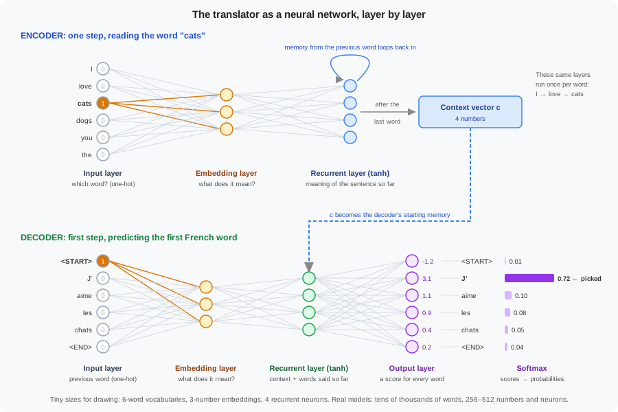
We’ll use a pretend world with only 6 English words and 6 French words, embeddings of 3 numbers, and a recurrent layer of 4 neurons. Real models are much bigger, but the layers are exactly the same.
The encoder’s layers
Layer 1 — Input layer: “Which word is this?”
The input layer has one neuron per word in the vocabulary. To feed in a word, we switch its neuron on (1) and every other neuron off (0). This is called one-hot encoding:
English vocabulary:   I   love   cats   dogs   you   the
Token ID:             0     1      2      3     4     5
"cats" goes in as:  [ 0,   0,     1,     0,     0,    0 ]
- In: the word’s fixed token ID from the vocabulary
- Out: 6 numbers, a single 1 and the rest 0s
- Adds: only identity. It says which word this is, but nothing about what it means. “cats” and “dogs” look just as different as “cats” and “the”.
- Learned weights: none. It’s just a switchboard.
In a real model the vocabulary might have 10,000 words, so the input layer has 10,000 neurons with exactly one of them on. (In code, libraries skip building this long list and just pass the word’s index, but the idea is the same.)
Layer 2 — Embedding layer: “What does this word mean?”
Every input neuron connects to every embedding neuron. The weights on those connections form the embedding matrix, one row of 3 numbers per vocabulary word:
Embedding matrix (6 words × 3 numbers), learned in training:

          e1      e2      e3
I      [ 0.12   -0.45    0.78 ]
love   [ 0.91    0.02   -0.64 ]
cats   [ 0.34    0.88    0.21 ]   ← similar to "dogs"
dogs   [ 0.30    0.85    0.25 ]   ← similar to "cats"
you    [ 0.15   -0.40    0.70 ]   ← similar to "I"
the    [ 0.05    0.10    0.02 ]
Each embedding neuron adds up (input × weight) over all 6 inputs. Because only “cats” is 1 and everything else is 0, every row except the “cats” row gets multiplied by 0 and disappears:
e1 = 0×0.12 + 0×0.91 + 1×0.34 + 0×0.30 + 0×0.15 + 0×0.05 = 0.34
e2 = ...                1×0.88 ...                      = 0.88
e3 = ...                1×0.21 ...                      = 0.21

"cats" → [0.34, 0.88, 0.21]     (exactly the "cats" row)
So the embedding layer is simply “look up the word’s row”. That is the same lookup we did in section 4, now seen as a layer of neurons.
- In: the one-hot vector (6 numbers)
- Out: 3 meaningful numbers
- Adds: meaning. Words used in similar ways get similar numbers, so “cats” is now close to “dogs” and “I” is close to “you”. (That’s all of Part 1, in one layer.)
- Learned weights: the embedding matrix (6 × 3 = 18 weights). There’s no activation function, so it’s a pure lookup.
Layer 3 — Recurrent layer: “What does the sentence mean so far?”
This is the hidden layer with the loop from section 5. Each of its 4 neurons receives 7 inputs:
- the 3 numbers from the embedding layer (the current word)
- its own 4 outputs from the previous word (the memory)
Each neuron multiplies every input by a weight, adds them up with a bias, and squashes the total with tanh:
h_t = tanh(W_x × x_t + W_h × h_{t-1} + b)
The fully worked example with real numbers is in section 5.
- In: the word’s 3 embedding numbers + the previous 4 memory numbers
- Out: 4 new memory numbers (the hidden state)
- Adds: memory and order. This is the only layer that knows what came before. After “cats”, its 4 numbers describe “I love cats”, not just “cats”.
- Learned weights:
W_x(3 × 4 = 12),W_h(4 × 4 = 16) andb(4), so 32 in total.
The encoder runs layers 1 → 2 → 3 once per word, reusing the same weights each time. After the last word, the recurrent layer’s 4 numbers are the context vector.
If the encoder has stacked recurrent layers (section 5), each extra layer takes the 4 numbers from the layer below as its input and adds deeper patterns, such as phrases and overall meaning rather than single words.
No output layer
The encoder never has to name a word, so it needs no output layer. Its only product is the context vector.
The decoder’s layers
Layer 1 — Input layer: “Which word did I just say?”
Same idea as the encoder’s input layer, but over the French vocabulary. At the very first step there’s no previous word yet, so we switch on the special <START> neuron:
French vocabulary:  <START>   J'   aime   les   chats   <END>
first step:        [   1,      0,    0,    0,     0,      0   ]
- Adds: identity of the previous word (or “we’re just starting”).
- Learned weights: none.
Layer 2 — Embedding layer: “What does that word mean?”
It works exactly like the encoder’s embedding layer, but with its own French embedding matrix (6 × 3).
- Adds: meaning of the previous French word.
- Learned weights: the French embedding matrix.
Layer 3 — Recurrent layer: “What have I said, and what was the input about?”
It’s the same kind of layer as in the encoder, with its own W_x, W_h and b. There’s one big difference: its memory does not start at zeros. It starts as the context vector from the encoder.
- In: the previous word’s 3 embedding numbers + 4 memory numbers (the context vector at step 1)
- Out: 4 new memory numbers
- Adds: the link between what the input sentence meant and what has been written so far.
- Learned weights: 32 (its own set).
Layer 4 — Output layer: “How good is each possible next word?”
The output layer has one neuron per French word. Each is connected to all 4 recurrent neurons, and each produces one score (also called a logit). There’s no tanh here: the scores can be any size.
<START>   J'    aime   les    chats   <END>
 -1.2    3.1    1.1    0.9    0.4     0.2
- In: 4 memory numbers
- Out: 6 scores, one per French word
- Adds: a vote for every possible next word.
- Learned weights: 4 × 6 = 24 weights + 6 biases = 30.
Layer 5 — Softmax: “How sure am I?”
Softmax turns the scores into probabilities that add up to 1. It makes each score positive with e^score, then divides by the total:
word       score    e^score    ÷ total (30.67)
<START>    -1.2       0.30       0.01
J'          3.1      22.20       0.72   ← highest, so pick "J'"
aime        1.1       3.00       0.10
les         0.9       2.46       0.08
chats       0.4       1.49       0.05
<END>       0.2       1.22       0.04
                    ------      -----
                     30.67       1.00
- Adds: confidence. The model now says “72% sure the first word is J’”.
- Learned weights: none. Softmax is a fixed formula.
The decoder outputs “J’“. At the next step, “J’” is switched on in the decoder’s input layer, and all five layers run again, until the model picks <END>.
All the layers on one page
| # | Layer | Neurons (toy → real) | What goes in | What comes out | What it adds | Learned? |
|---|---|---|---|---|---|---|
| E1 | Encoder input | 6 → ~10,000 | A word | One-hot (single 1) | Which word | No |
| E2 | Encoder embedding | 3 → 256 | One-hot | Word vector | Meaning of the word | Yes: embedding matrix |
| E3 | Encoder recurrent | 4 → 512 | Word vector + own memory | New memory | Order and memory of the sentence | Yes: W_x, W_h, b |
| — | Context vector | 4 → 512 | Final memory | Same numbers | The hand-off to the decoder | No (just copied) |
| D1 | Decoder input | 6 → ~12,000 | Previous word | One-hot | Which word was just said | No |
| D2 | Decoder embedding | 3 → 256 | One-hot | Word vector | Meaning of that word | Yes: its own embedding matrix |
| D3 | Decoder recurrent | 4 → 512 | Word vector + memory (starts as context) | New memory | Links input meaning to output so far | Yes: its own W_x, W_h, b |
| D4 | Output layer | 6 → ~12,000 | Memory | One score per word | A vote for every next word | Yes: output weights + bias |
| D5 | Softmax | 6 → ~12,000 | Scores | Probabilities | Confidence (adds to 1) | No |
Following the sizes through the network
ENCODER (runs once per input word)
  word "cats"
    → input layer        [6]     one-hot
    → embedding layer    [3]     meaning
    → recurrent layer    [4]     meaning so far   ──┐ loops back for the next word
                                                    │
  after the last word:   context vector [4] ────────┘
                                   │
DECODER (runs once per output word)│
  previous word "<START>"          │
    → input layer        [6]       │
    → embedding layer    [3]       ↓
    → recurrent layer    [4]   ← starts from the context vector
    → output layer       [6]     one score per French word
    → softmax            [6]     probabilities → pick "J'"
How many weights is that?
| Part | Toy model | Real model (10k English words, 12k French, 256 embedding, 512 neurons) |
|---|---|---|
| Encoder embedding | 6 × 3 = 18 | 10,000 × 256 = 2,560,000 |
Encoder recurrent (W_x + W_h + b) |
12 + 16 + 4 = 32 | 131,072 + 262,144 + 512 = 393,728 |
| Decoder embedding | 6 × 3 = 18 | 12,000 × 256 = 3,072,000 |
| Decoder recurrent | 32 | 393,728 |
| Output layer (weights + bias) | 24 + 6 = 30 | 6,144,000 + 12,000 = 6,156,000 |
| Total | 130 | ≈ 12.6 million |
Two things stand out. The embedding and output layers hold most of the weights, because they have one row or neuron per vocabulary word. And the recurrent layers are small but do the “thinking”. (An LSTM or GRU has about 3–4 times more recurrent weights than this plain RNN, but the same layer structure.)
Where does training fit in?
The loss is measured at the very end, by comparing softmax’s probabilities with the correct word (section 11). Backpropagation then walks backwards through the layers, nudging every learned weight on the way:
softmax → output layer → decoder recurrent → decoder embedding
                               ↓
                        context vector
                               ↓
                encoder recurrent → encoder embedding
The input layers and softmax have nothing to learn, so the error just passes through them. Every other layer in the table gets a little better with each training example.
10. A concrete example: English → French
Let’s walk through translating “I love cats” to “J’aime les chats.”
Encoder
Word       Embedding          Hidden state
─────────  ─────────────────  ──────────────
"I"        [0.1, 0.3, ...]   h1 = tanh(W_h·h0 + W_x·emb("I") + b)
"love"     [0.8, -0.2, ...]  h2 = tanh(W_h·h1 + W_x·emb("love") + b)
"cats"     [0.4, 0.7, ...]   h3 = tanh(W_h·h2 + W_x·emb("cats") + b)

Context vector c = h3
Decoder
Input token    Hidden state               Softmax output     Predicted word
─────────────  ─────────────────────────  ─────────────────  ──────────────
<START>        s1 = tanh(W·c + W·emb(<START>) + b)          "J'"
"J'"           s2 = tanh(W·s1 + W·emb("J'") + b)           "aime"
"aime"         s3 = tanh(W·s2 + W·emb("aime") + b)         "les"
"les"          s4 = tanh(W·s3 + W·emb("les") + b)          "chats"
"chats"        s5 = tanh(W·s4 + W·emb("chats") + b)        <END>
11. Loss function: cross-entropy
At each decoder step, the network predicts a probability distribution over the entire vocabulary. The loss measures how far that distribution is from the correct word.
At step 2, the correct word is "aime".
The model predicts: P("aime") = 0.7, P("adore") = 0.15, P("chat") = 0.05, ...

Cross-entropy loss = -log(0.7) = 0.36
The total loss for the sentence is the sum (or average) of the losses at each step. Backpropagation flows through the decoder, through the context vector, and back into the encoder — so both halves learn together.
12. Common applications
| Task | Input | Output |
|---|---|---|
| Machine translation | “I love cats” | “J’aime les chats” |
| Text summarisation | A long article | A short summary |
| Chatbot | User message | Bot reply |
| Text-to-SQL | “Show me all users over 30” | SELECT * FROM users WHERE age > 30 |
| Image captioning | An image (CNN features) | “A dog running on a beach” |
In image captioning, the encoder is a CNN instead of an RNN — it compresses the image into a vector. The decoder is still an RNN that generates text.
13. PyTorch sketch
import torch
import torch.nn as nn

class Encoder(nn.Module):
    def __init__(self, vocab_size, embed_dim, hidden_dim):
        super().__init__()
        self.embedding = nn.Embedding(vocab_size, embed_dim)
        self.rnn = nn.GRU(embed_dim, hidden_dim, batch_first=True)

    def forward(self, x):
        embedded = self.embedding(x)          # (batch, seq_len, embed_dim)
        outputs, hidden = self.rnn(embedded)  # hidden = context vector
        return hidden                         # (1, batch, hidden_dim)

class Decoder(nn.Module):
    def __init__(self, vocab_size, embed_dim, hidden_dim):
        super().__init__()
        self.embedding = nn.Embedding(vocab_size, embed_dim)
        self.rnn = nn.GRU(embed_dim, hidden_dim, batch_first=True)
        self.fc = nn.Linear(hidden_dim, vocab_size)

    def forward(self, x, hidden):
        embedded = self.embedding(x)          # (batch, 1, embed_dim)
        output, hidden = self.rnn(embedded, hidden)
        prediction = self.fc(output)          # (batch, 1, vocab_size)
        return prediction, hidden
The encoder reads the full input and returns a hidden state. The decoder takes that hidden state and generates one word per call.
14. Summary
- The encoder reads the input sequence and compresses it into a context vector.
- The decoder starts from the context vector and generates the output sequence one word at a time.
- As a neural network, each side is a stack of layers: input (which word) → embedding (what it means) → recurrent (what the sentence means so far), and the decoder adds an output layer (a score per word) and softmax (probabilities).
- During training, teacher forcing feeds the correct previous word to the decoder; during inference, the model uses its own predictions.
- The loss is cross-entropy at each output step, and backpropagation trains both encoder and decoder together.
- This architecture powers translation, summarisation, chatbots, and more.
- The main weakness is that the entire input is squeezed into one fixed-size vector — long sentences lose information. The next part shows how attention fixes this.