
Computer Vision - Part 6: Region-Based Object Detectors
Computer Vision — Part 6: Region-Based Object Detectors
One way to find objects is to ask: “What regions of the image might contain something interesting?” If we can answer that question first, we only need to run an expensive classifier on a small number of candidate regions. Detectors that follow this idea are called region-based detectors.
This part explains the R-CNN family from the first version to Faster R-CNN and shows why they dominated object detection for several years.
1. The core problem
A photo has millions of pixels. Objects can appear anywhere and at any size.
The naive solution would be:
- Cut every possible rectangle out of the image.
- Run a classifier on every rectangle.
- Keep the rectangles that are confidently a known object.
The number of possible rectangles is enormous. For a normal photo there can be millions. Running a CNN millions of times is far too slow.
Region-based detectors solve this by proposing a small number of promising regions first, then classifying only those regions.

2. R-CNN (2014)
R-CNN stands for Regions with CNN features. It was the first successful deep-learning approach to object detection.
Pipeline
1. Input image
2. Run Selective Search to find about 2,000 candidate regions
3. Crop and warp each region to a fixed size (e.g. 227 × 227)
4. Run a CNN on each cropped region to extract features
5. Run an SVM classifier on the features to get the class
6. Run a linear regression to refine the box
Why it was important
Before R-CNN, object detection relied on hand-designed features. R-CNN showed that features learned by a CNN, pretrained on ImageNet, could dramatically improve accuracy.
Limitations
| Limitation | Why it hurts |
|---|---|
| Slow training | Thousands of crops had to be stored on disk. |
| Slow inference | The CNN runs ~2,000 times per image. |
| Not end-to-end | The CNN, SVM, and bounding-box regressor were trained separately. |
| Fixed-size warping | Objects were distorted to fit the CNN input. |
R-CNN was accurate, but it was too slow for real-time use.
3. Fast R-CNN (2015)
Fast R-CNN fixed the biggest speed problem of R-CNN: it ran the CNN once instead of thousands of times.
The key insight
A CNN produces a feature map — a smaller, dense representation of the whole image. Cropping a region from the original image and running it through the CNN gives a very similar result to cropping the same region directly from the feature map.
So Fast R-CNN does:
1. Run the whole image through a CNN once → feature map
2. Use Selective Search to get ~2,000 region proposals
3. For each proposal, crop the matching patch from the feature map
4. Run a small classifier and box regressor on each patch
RoI pooling
Feature maps are smaller than the original image. A proposal rectangle must be mapped to the feature-map coordinates. RoI pooling (Region of Interest pooling) crops the matching patch and resizes it to a fixed size so the next layers always receive the same shape.
Original image:        800 × 600
CNN stride:            16
Feature map:           50 × 37.5  → rounded to 50 × 38
A proposal (160, 120, 320, 240) maps to (10, 7, 20, 15) in the feature map
RoI pool it to a fixed 7 × 7 patch
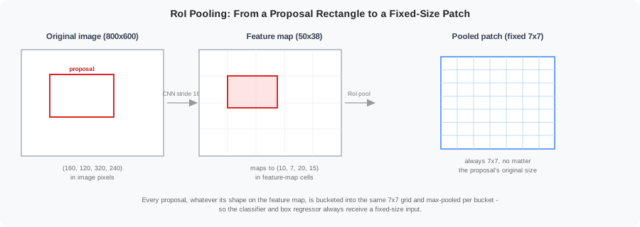
Every proposal is divided into the same number of buckets (7 × 7 here), and each bucket is max-pooled down to one value — a big proposal and a tiny proposal both end up as a 7 × 7 patch, just pooled over regions of different sizes.
Benefits over R-CNN
| R-CNN | Fast R-CNN |
|---|---|
| CNN runs ~2,000 times | CNN runs 1 time |
| Multi-stage training | Joint end-to-end training |
| Features stored on disk | Everything stays in memory |
| Much slower | Significantly faster |
Remaining bottleneck
Selective Search still takes about 2 seconds per image and cannot run on a GPU. It became the new slowest part of the pipeline.
4. Faster R-CNN (2015)
Faster R-CNN removed Selective Search entirely. It asked the network itself to propose regions.
The big idea
If the CNN already looks at the whole image to build a feature map, why not also use that feature map to predict which rectangles are worth checking?
The new module that does this is called the Region Proposal Network (RPN).
Faster R-CNN pipeline
Image → shared CNN backbone → shared feature map
                                  ↓
                    ┌──────────────┴──────────────┐
                    ↓                             ↓
            Region Proposal Network (RPN)    detection head
                    ↓                             ↓
            candidate boxes                  class + refined boxes
The RPN and the detection head share the same feature map, so the expensive CNN computation only happens once.
5. Region Proposal Network (RPN)
The RPN slides a small network over the shared feature map. At every location it evaluates anchor boxes of different sizes and shapes.

Anchors
At each feature-map cell, the RPN tries 9 anchors by default:
- 3 sizes: small, medium, large
- 3 aspect ratios: 1:1, 1:2, 2:1
3 sizes × 3 ratios = 9 anchors
For each anchor, the RPN outputs:
- Objectness score — is there probably an object here?
- Box regression — how should this anchor be shifted or resized to fit the real object?
The RPN does not say what the object is. It only says “object vs. not object” and where the box should be.
Non-Maximum Suppression in the RPN
The RPN can produce tens of thousands of candidate boxes. Most overlap heavily. Non-Maximum Suppression (NMS) keeps only the best box from each cluster.
1. Sort all boxes by objectness score
2. Pick the highest-scoring box
3. Remove boxes that overlap it too much (IoU > threshold, usually 0.7)
4. Repeat until no boxes remain
After NMS, around 300 candidate boxes remain and are passed to the detection head.
6. Two-stage training
Faster R-CNN has four loss terms that are trained jointly:
L = L_rpn_cls + L_rpn_reg + L_cls + L_reg
| Loss | Meaning |
|---|---|
| L_rpn_cls | RPN objectness: is this anchor an object or background? |
| L_rpn_reg | RPN box refinement for positive anchors |
| L_cls | Final classifier: what class is the object? |
| L_reg | Final box refinement for detected objects |
In practice, training is done in alternating steps or with approximate joint training, but modern implementations train everything end-to-end.
7. Fully convolutional networks and detection
Modern detection networks are usually fully convolutional: every layer is a convolution. There are no fully-connected layers at the end.
Why this matters:
- A fully-connected layer requires a fixed input size. A fully convolutional network accepts any input size.
- Feature maps keep spatial information, which is exactly what detection needs.
- Faster R-CNN is fully convolutional up to the RoI pooling layer.
The RPN is itself fully convolutional: a small 3 × 3 convolution slides over the feature map, and two 1 × 1 convolution heads produce objectness and box regression outputs.
Shared feature map (H × W × C)
    ↓ 3 × 3 conv
Intermediate features
    ↓ 1 × 1 conv  → objectness scores  (H × W × 2k)
    ↓ 1 × 1 conv  → box regressions    (H × W × 4k)
Here k is the number of anchors per cell, usually 9.
8. Limitations of region-based methods
Faster R-CNN is accurate, but it still has drawbacks:
| Limitation | Explanation |
|---|---|
| Two-stage pipeline | Propose regions first, then classify. This adds latency. |
| Slow for real-time | Typical speed is 5-17 frames per second on a GPU. |
| Anchor design | Anchor sizes and ratios must be tuned for the dataset. |
| Small objects | Tiny objects may be missed because they occupy few feature-map cells. |
| RoI pooling loses precision | Quantising box coordinates to the feature grid loses sub-pixel accuracy. |
RoIAlign, introduced in Mask R-CNN, fixed the quantisation problem by using bilinear interpolation instead of rounding. This is especially important for instance segmentation.
9. Run Faster R-CNN in PyTorch
import torch
import torchvision
from torchvision.models.detection import fasterrcnn_resnet50_fpn
from torchvision.transforms import functional as F
from PIL import Image

# Load a pretrained model
model = fasterrcnn_resnet50_fpn(pretrained=True)
model.eval()

# Load an image
image = Image.open("street.jpg").convert("RGB")
image_tensor = F.to_tensor(image)

# Run inference
with torch.no_grad():
    predictions = model([image_tensor])

# predictions[0] is a dictionary with boxes, labels, scores
boxes   = predictions[0]["boxes"]
labels  = predictions[0]["labels"]
scores  = predictions[0]["scores"]

# Show results above a confidence threshold
for box, label, score in zip(boxes, labels, scores):
    if score > 0.5:
        print(f"Label {label.item()}: {box.tolist()}  score={score.item():.2f}")
The model returns COCO class indices, so label values map to classes such as person, car, dog, etc.
10. Summary
- Region-based detectors first propose a small set of candidate regions, then classify them.
- R-CNN used Selective Search and ran a CNN thousands of times. Accurate but slow.
- Fast R-CNN ran the CNN once and used RoI pooling. Still relied on slow Selective Search.
- Faster R-CNN replaced Selective Search with the Region Proposal Network (RPN), making proposals nearly free.
- The RPN uses anchor boxes and produces objectness scores and box regressions.
- Region-based detectors are accurate but slower than one-stage detectors.
- Fully convolutional designs and shared feature maps are the key to efficient detection.
Next: Part 7: Anchor Boxes