
Computer Vision - Part 4: Object Detection Basics
Computer Vision — Part 4: Object Detection Basics
In the previous part we learned that computer vision lets machines understand images. One of the most important tasks is object detection: finding every object in an image, drawing a box around it, and saying what it is.
This part explains the building blocks of detection: bounding boxes, coordinates, how a detector is structured, and the main metrics used to check its quality.
1. What is object detection?
Image classification asks: what is in this image? It gives one answer for the whole picture.
Object localisation asks: where is the main object? It gives one box around the main object.
Object detection asks: what objects are in the image and where are they? It gives a list of boxes and labels.
Classification:  "There is a cat in this image."
Localisation:    "The cat is inside the box (50, 30, 200, 180)."
Detection:       "Cat at (50, 30, 200, 180) with confidence 0.95,
                   Dog at (220, 90, 400, 250) with confidence 0.87"
2. Bounding boxes
A bounding box is the rectangle that tightly contains an object. It is the most common way to say “it is here” in object detection.
Two popular ways to write a box:
| Format | Meaning | Example |
|---|---|---|
(x, y, w, h) |
top-left corner plus width and height | (50, 30, 150, 150) |
(x1, y1, x2, y2) |
top-left and bottom-right corners | (50, 30, 200, 180) |
The two formats are easy to convert:
x2 = x + w
y2 = y + h

w  = x2 - x
h  = y2 - y
Corner coordinates are useful for drawing

Coordinates are usually measured in pixels, with (0, 0) at the top-left of the image and y increasing downward.
3. Object localisation
Object localisation is the simpler version of detection. There is assumed to be exactly one main object in the image, and the job is to find its box.
The output usually has two parts:
- A class label — what the object is.
- A bounding box — where the object is.
This is common in robotics and industrial inspection when you know one item is in front of the camera.
4. The object detection pipeline
A modern detector follows a small number of clear steps:
→ feature maps"] B --> C["Detection head
→ raw box coordinates and class scores"] C --> D["Postprocessing
→ keep only the best boxes (NMS)"] D --> E["Final predictions"] classDef step fill:#dbeafe,stroke:#1d4ed8,stroke-width:1.5px,color:#111 class A,B,C,D,E step
Backbone
The backbone is a CNN such as ResNet or VGG. It turns the input image into a smaller set of feature maps. You can think of these as a summary of what the image contains at many locations.
Detection head
The head takes the feature maps and produces raw predictions. For every candidate location, it outputs:
- box coordinates
- objectness score (is there an object?)
- class probabilities (what kind of object?)
Postprocessing
Many nearby candidates may point to the same real object. Non-Maximum Suppression (NMS) removes duplicates by keeping the box with the highest score and deleting overlapping boxes.
5. Why is object detection hard?
Detection is harder than classification because the computer must answer two questions at once:
- Where? — it must scan many locations and scales.
- What? — it must classify each candidate.
Extra difficulties:
| Difficulty | Explanation |
|---|---|
| Many objects | An image can contain 0, 1, or hundreds of objects. |
| Different sizes | The same object can be tiny or huge in the photo. |
| Different shapes | Cars are wide, people are tall, plates are round. |
| Overlap | Objects can hide or partially cover each other. |
| Background confusion | A brown box may look like a parcel or a dog. |
| Speed | Real-time video needs 30 or more detections per second. |
6. Intersection over Union (IoU)
To know whether a predicted box is good, we compare it with the ground-truth box drawn by a human. The most common comparison is IoU.
              area of overlap
IoU = ─────────────────────────────
       area of union of both boxes
              |A ∩ B|
IoU(A, B) = ───────────
              |A ∪ B|
If the boxes perfectly overlap, IoU is 1.0. If they do not overlap at all, IoU is 0.0.
Worked example
Box A (predicted): (10, 10, 60, 60) → width 50, height 50, area 2500.
Box B (ground truth): (30, 30, 80, 80) → width 50, height 50, area 2500.
The boxes overlap from (30, 30) to (60, 60), so the overlap is 30 × 30 = 900.
The union is 2500 + 2500 - 900 = 4100.

IoU = 900 / 4100 ≈ 0.22
A common rule is: if IoU ≥ 0.5, the prediction is counted as a true positive.
import numpy as np

def iou(box_a, box_b):
    """
    box = [x1, y1, x2, y2]
    """
    x1 = max(box_a[0], box_b[0])
    y1 = max(box_a[1], box_b[1])
    x2 = min(box_a[2], box_b[2])
    y2 = min(box_a[3], box_b[3])

    inter_width  = max(0, x2 - x1)
    inter_height = max(0, y2 - y1)
    inter_area   = inter_width * inter_height

    area_a = (box_a[2] - box_a[0]) * (box_a[3] - box_a[1])
    area_b = (box_b[2] - box_b[0]) * (box_b[3] - box_b[1])

    union_area = area_a + area_b - inter_area

    return inter_area / union_area if union_area > 0 else 0.0

predicted = [10, 10, 60, 60]
ground    = [30, 30, 80, 80]
print(iou(predicted, ground))  # about 0.22
7. Precision, recall, and Average Precision (AP)
A detector can make two kinds of mistakes:
- False positive — it says an object is there, but it is not.
- False negative — it misses a real object.
                 true positives
Precision = ─────────────────────────────
             true positives + false positives

                 true positives
Recall = ─────────────────────────────
          true positives + false negatives
- A model with high precision rarely cries wolf.
- A model with high recall rarely misses things.
If we sort all predictions by confidence and plot precision against recall, the area under the curve is called Average Precision (AP). It summarises how well the detector finds one class.
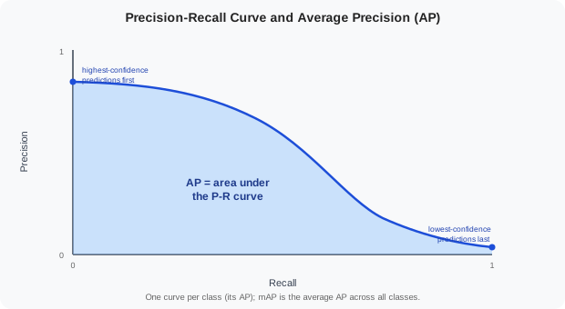
Mean Average Precision (mAP) is the average AP over all object classes. It is the standard score for comparing object detectors.
mAP = (AP for class 1 + AP for class 2 + ... + AP for class K) / K
8. Two-stage vs one-stage detectors
Detectors are grouped into two families:
| Family | Idea | Speed | Typical models |
|---|---|---|---|
| Two-stage | First propose regions, then classify each region. | Slower, usually more accurate | R-CNN, Fast R-CNN, Faster R-CNN |
| One-stage | Predict boxes and classes in a single forward pass. | Faster, often slightly less accurate | YOLO, SSD, RetinaNet, DETR |
A two-stage detector is like an editor who first lists story ideas and then writes each article. A one-stage detector is like a reporter who writes the headline and the story at the same time.
9. Summary
- Object detection finds objects, draws boxes, and labels them.
- Object localisation finds the box for a single main object.
- A bounding box can be written as
(x, y, w, h)or(x1, y1, x2, y2). - The detection pipeline is: image → backbone → detection head → NMS → predictions.
- IoU measures how much a predicted box overlaps the ground truth.
- Precision and recall measure correctness and completeness.
- mAP is the standard metric for detector quality.
- Detectors are either two-stage or one-stage.