Computer Vision — Part 1: Image Processing Fundamentals

Before a computer can generate or understand images, it must learn to read them. The first step is to stop seeing an image as a picture and start seeing it as a grid of numbers.

This lesson explains how digital images are stored, how colour works, how we change images with small mathematical operations, and how convolution helps us find edges and other patterns.

1. A digital image is a grid of numbers

A digital image is a grid of tiny squares called pixels. Each pixel stores a number that represents brightness or colour.

Binary images

The simplest image is binary: every pixel is either 0 (black) or 1 (white).

0 0 1 1 0 0
0 1 0 0 1 0
0 1 1 1 1 0
0 1 0 0 1 0
0 1 0 0 1 0

This grid is the letter A. You can see the shape because the 1s form lines.

Grayscale images

A grayscale image uses one number per pixel, usually from 0 to 255.

• 0 = pure black
• 255 = pure white
• The numbers in between = different shades of grey

If the grid above used 0 to 255 instead of 0 to 1, the idea would be the same. The darker the pixel, the smaller the number. The brighter the pixel, the larger the number.

Colour images

A colour image has three numbers per pixel instead of one. The most common model is RGB.

• R = Red
• G = Green
• B = Blue

Each channel is also from 0 to 255. By mixing different amounts of red, green and blue, you can create almost any colour.

pixel = [255, 0, 0]    # pure red
pixel = [0, 255, 0]    # pure green
pixel = [0, 0, 255]    # pure blue
pixel = [255, 255, 255] # white
pixel = [0, 0, 0]      # black

The floor-tile analogy

Think of an image as a wall made of floor tiles. Each tile is one pixel.

• A grayscale wall has one number painted on each tile.
• A colour wall has three numbers painted on each tile: how much red, how much green, how much blue.
• A video is just many walls shown one after another.

2. Image dimensions: height, width and channels

When we describe the size of an image in code, we use three numbers:

(height, width, channels)

• Height = number of rows of pixels.
• Width = number of columns of pixels.
• Channels = how many numbers each pixel carries.

A typical image might have shape (480, 640, 3):

• 480 rows
• 640 columns
• 3 colour channels (RGB)

A grayscale image has shape (480, 640, 1) because it has only one channel.

import numpy as np

# A tiny 4x4 grayscale image
gray = np.array([
    [0, 50, 100, 150],
    [50, 100, 150, 200],
    [100, 150, 200, 250],
    [150, 200, 250, 255]
])

print(gray.shape)  # (4, 4)

# A tiny 2x2 colour image
rgb = np.array([
    [[255, 0, 0], [0, 255, 0]],
    [[0, 0, 255], [255, 255, 255]]
])

print(rgb.shape)  # (2, 2, 3)

3. Common colour models

A colour model is a way to describe colour with numbers.

RGB

RGB is the default for screens and cameras. It uses red, green and blue channels.

It is an additive model. Add more light and the colour gets brighter. All three at full strength make white.

CMYK

CMYK is used for printing. It stands for Cyan, Magenta, Yellow and Key (black).

It is a subtractive model. You start with white paper and add ink. The more ink, the darker the result. It is not usually needed for on-screen work.

HSV

HSV is closer to how humans think about colour.

• H = Hue. The name of the colour: red, orange, blue.
• S = Saturation. How pure the colour is. 0 is grey, 255 is vivid.
• V = Value. How bright the colour is. 0 is black, 255 is full brightness.

HSV is useful when you want to change a colour without changing its brightness, or when you want to pick every shade of blue from an image.

4. Basic arithmetic on images

Because an image is a matrix, we can do normal math on it.

Addition: blending two images

Adding two images pixel by pixel makes a blended image.

new_pixel = pixel_image_1 + pixel_image_2

If both pixels are bright, the result is very bright. This is useful for overlays and double-exposure effects.

Subtraction: finding the difference

Subtracting one image from another shows what changed.

new_pixel = pixel_image_1 - pixel_image_2

If a security camera takes two pictures and nothing moved, the result is close to black. If a person walked in, those pixels will show a large difference. This is how motion detection often starts.

Multiplication and division: brightness control

Multiplying every pixel by a number makes the image brighter. Dividing makes it darker.

bright = pixel * 1.5
dark   = pixel * 0.5

Values above 255 are usually clipped back to 255, otherwise the image would wrap around and look strange.

Logical operations: masks

A mask is a binary image that says “keep these pixels, ignore the others.”

With a bitwise AND, you can cut out a region of interest. With a bitwise OR, you can combine shapes.

This is like using a stencil when spray-painting. The stencil decides where the paint goes.

5. Filters and transformations

A filter is a small grid of numbers called a kernel. We move this kernel over the image and compute a new value for each pixel.

Filters can blur, sharpen, detect edges or remove noise.

The recipe-card analogy

Imagine you are looking at a photograph through a small square magnifying glass. The magnifying glass only shows a 3x3 patch at a time. You write a rule for how to mix the nine pixel values you see into one new value. Then you slide the glass across the whole image and repeat.

That rule is the kernel.

Sharpening

A common sharpening trick is:

sharpened = original + (original - blurred)

First, create a slightly blurred copy. Then subtract the blurred copy from the original. This gives you the fine details. Add those details back to the original image and the result looks sharper.

You can also write this as a single 3x3 kernel:

 0  -1   0
-1   5  -1
 0  -1   0

When this kernel is applied, the center pixel is boosted and the neighbours are reduced. This makes edges stand out.

6. Convolution step by step

Convolution is the name for the slide-multiply-sum operation used to apply a kernel.

Here is how it works on a 3x3 patch of an image.

Input patch

10  20  30
40  50  60
70  80  90

Kernel

0  1  0
1 -4  1
0  1  0

Multiply each value by the kernel value

10×0   20×1   30×0    =   0  20   0
40×1   50×-4  60×1    =  40 -200 60
70×0   80×1   90×0    =   0  80   0

Add everything up

0 + 20 + 0 + 40 + (-200) + 60 + 0 + 80 + 0 = 0

The output pixel for the center position is 0.

This particular kernel finds edges. When the centre is very different from its neighbours, the result is a large positive or negative number. When the neighbourhood is flat, the result is near zero.

Sliding across the image

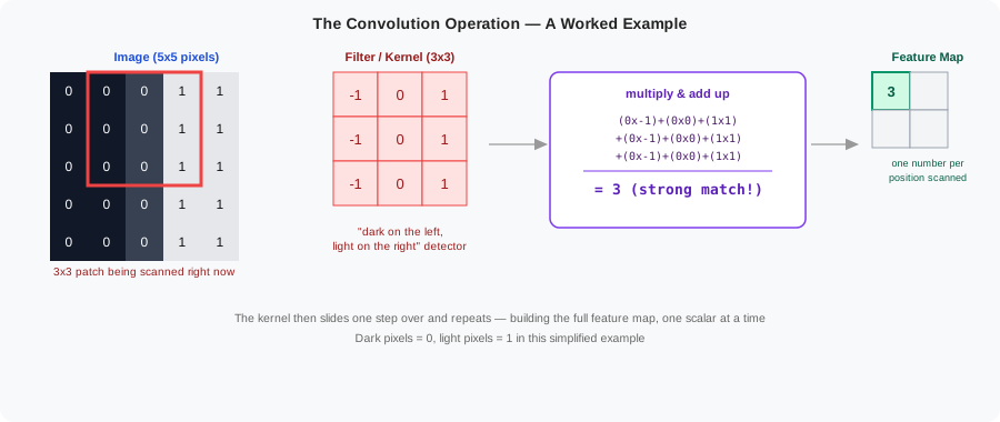
We place the kernel over every pixel, compute the sum, and write the result into a new image. Pixels at the border are special because the kernel would hang over the edge. There are two common fixes:

1. Ignore the border. The output image becomes slightly smaller.
2. Add padding. We place a ring of extra pixels, usually zeros, around the input image so the kernel can reach the edge.

The second option is called padding. With a 3x3 kernel and padding of 1, the output image keeps the same size as the input.

7. Why convolution is powerful

Convolution does three useful things at once.

1. Feature detection. It can highlight edges, corners, lines or textures depending on the kernel.
2. Noise reduction. Some kernels smooth the image and hide small random changes.
3. Compact representation. The output is often smaller and more meaningful than the raw image.

This is why almost every computer vision model, from simple OpenCV scripts to deep neural networks, uses some form of convolution.

8. Common filters

Box blur / average filter

Every output pixel is the average of its neighbours. This smooths the image but can make edges fuzzy.

1/9  1/9  1/9
1/9  1/9  1/9
1/9  1/9  1/9

The 1/9 keeps the overall brightness the same.

Gaussian blur

A Gaussian blur uses weights shaped like a bell curve. The centre pixel matters most, and pixels farther away matter less. This looks more natural than a box blur.

A common 3x3 version is:

1/16  2/16  1/16
2/16  4/16  2/16
1/16  2/16  1/16

The 1/16 factor makes sure the image does not get brighter or darker.

Sobel edge detector

The Sobel filter finds edges by measuring how quickly brightness changes.

It uses two kernels:

Horizontal edges (Gx)      Vertical edges (Gy)
-1  0  1                   -1 -2 -1
-2  0  2                    0  0  0
-1  0  1                    1  2  1

One kernel is sensitive to horizontal changes, the other to vertical changes. The final edge strength is:

edge_strength = sqrt(Gx² + Gy²)

If both Gx and Gy are large, there is a strong edge. If both are small, the area is smooth.

Canny edge detector

Canny is a multi-step method, not a single kernel.

1. Blur the image with a Gaussian filter to remove noise.
2. Find gradients with Sobel.
3. Thin the edges to one pixel wide.
4. Classify pixels as strong edge, weak edge or non-edge using two thresholds.
5. Connect weak edges only if they touch strong edges.

Canny usually produces cleaner edges than a raw Sobel filter.

Median filter

A median filter is useful for removing speckled noise. It replaces the centre pixel with the median of its neighbours.

If the 3x3 neighbourhood is:

10  12  200
11  15  13
14  255  16

The sorted values are 10, 11, 12, 13, 14, 15, 16, 200, 255. The median is 14. So the centre pixel becomes 14 instead of 15.

The two extreme values 200 and 255 are ignored. This is why the median filter is so good at removing salt-and-pepper noise while keeping edges sharp.

9. Feature extraction

Feature extraction means finding the important parts of an image that help a model understand what is in it.

Low-level features

These are simple building blocks.

• Edges
• Corners
• Lines
• Textures
• Colours
• Basic shapes

These come directly from filters and convolutions.

High-level features

These are combinations of low-level features.

• A face is a combination of eyes, nose, mouth and edges.
• A car is a combination of wheels, windows, body shape and texture.

Classical computer vision hand-crafts these. Modern deep learning learns them automatically. Either way, the image must start as numbers first.

10. A quick look with OpenCV

OpenCV is a popular Python library for image processing. Here are a few one-line operations.

import cv2
import numpy as np

# Read a colour image
img = cv2.imread("photo.jpg")

# Convert to grayscale
gray = cv2.cvtColor(img, cv2.COLOR_BGR2GRAY)

# Gaussian blur
blur = cv2.GaussianBlur(img, (5, 5), 0)

# Canny edge detection
edges = cv2.Canny(gray, 100, 200)

# Median filter
median = cv2.medianBlur(img, 5)

The first argument of GaussianBlur is the image. The second is the kernel size, which must be an odd number. The third is the standard deviation; 0 lets OpenCV choose it automatically.

Canny takes two threshold values. Pixels above the upper threshold become strong edges. Pixels between the two thresholds become weak edges and are kept only if they connect to strong edges.

11. Summary

• A digital image is a grid of numbers.
• Grayscale images have one value per pixel. Colour images have three values per pixel, usually RGB.
• Image shape is (height, width, channels).
• You can add, subtract, multiply and divide images just like matrices.
• A kernel is a small grid of numbers. Convolution slides it over the image, multiplies, and sums.
• Common filters blur, sharpen, find edges or remove noise.
• Sobel finds edges by measuring brightness change in two directions.
• Canny cleans up edges with multiple steps.
• Median filter removes speckled noise without blurring edges.
• Features are the pieces of information an image contains, from edges to objects.

These ideas are the foundation of computer vision and of generative models that create or edit images. Every neural network that understands pictures begins by treating pixels as numbers.

Next: Part 2: Introduction