
Part 1: Understanding Neurons and Neural Networks - A Friendly Guide
Part 1: Understanding Neurons and Neural Networks — A Friendly Guide
Let us start with a real example instead of a formula.
Imagine a model that predicts whether an email is spam.
A human can read an email and notice things like:
- “This message contains too many links.”
- “The sender is unknown.”
- “It says WIN MONEY NOW.”
- “This looks suspicious.”
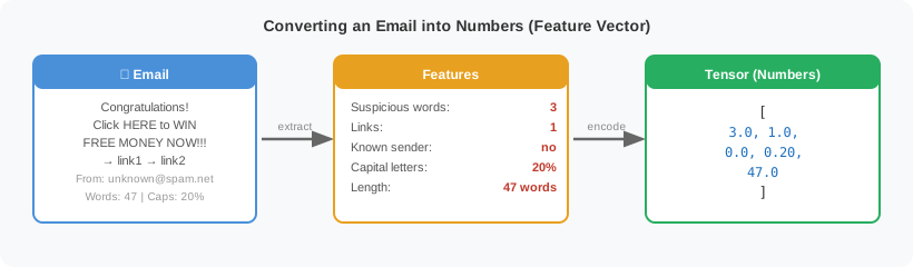
But a neural network cannot directly work with ideas such as suspicious, unknown sender, or too many links. A neural network performs mathematical operations: multiply, add, compare, transform. Therefore, the first job is to convert the email into numbers.
1. Why must everything become numbers?
A computer stores everything as numbers internally.
- An image becomes pixel values. A black pixel might be
0, a white pixel255. - Sound becomes measurements of air-wave amplitude.
- Words become token IDs or vectors.
An email can become measurable features such as:
- Number of suspicious words
- Number of links
- Sender known or unknown
- Percentage of capital letters
- Number of attachments
- Message length
The model does not receive this:
“Congratulations! Click here to claim your prize.”
A simple model may receive this:
| Suspicious words | Links | Known sender | Capitals | Length |
|---|---|---|---|---|
| 3 | 1 | no | 20% | 47 words |
Converted into numbers:
[3, 1, 0, 0.20, 47]
Who decides what counts as suspicious? In this simple model, a human does. A person might write a list of words like “win”, “free”, “prize”, and “money”, then count how many appear in the email. The neural network only learns how much weight to give that count. Later, in deep learning, the model can learn which words are suspicious directly from thousands of labelled emails.
This collection of numbers is called a feature vector. In PyTorch, it becomes a tensor:
import torch

email = torch.tensor([
    3.0,    # suspicious word count
    1.0,    # link count
    0.0,    # sender known: 0 = no, 1 = yes
    0.20,   # percentage of capital letters
    47.0    # message length
])
A tensor is simply a structured container of numbers.
Memory trick: A tensor is a lunchbox. The numbers are the food items, but each compartment has a fixed meaning.
2. What does each number mean?
The position of each number has a fixed meaning.
| Position | Meaning |
|---|---|
| 0 | suspicious words |
| 1 | links |
| 2 | known sender |
| 3 | capital-letter percentage |
| 4 | message length |
Therefore [3, 1, 0, 0.20, 47] does not mean anything by itself unless the model and the data-processing code agree on what each position represents. This is similar to a row in a table without the column headers.
3. Why use 0 and 1?
Some information is not naturally numerical. For example, known sender = yes or known sender = no. We convert it to:
- Yes = 1
- No = 0
This does not mean that “yes is greater than no” in a meaningful human sense. It is simply a convenient numerical representation.
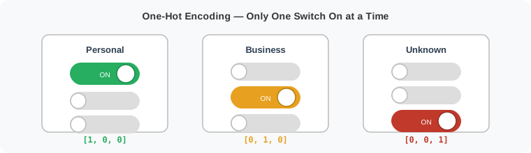
For multiple categories, we must be more careful. Suppose sender type is Personal, Business, or Unknown. Using Personal = 1, Business = 2, Unknown = 3 could accidentally suggest that Unknown is numerically greater than Business. Instead, we use one-hot encoding:
- Personal →
[1, 0, 0] - Business →
[0, 1, 0] - Unknown →
[0, 0, 1]
Memory trick: One-hot encoding is like three separate light switches. Only one is on at a time.
4. Does someone manually choose these features?
For a basic machine-learning model, yes. A developer or data scientist may decide to count suspicious words, count links, check sender reputation, measure capital letters, and measure message length. This is called feature engineering.
But modern deep-learning models can learn many features automatically. For example, instead of manually counting suspicious words, we can provide the email text as tokens. The sentence “claim your free prize” might become [1842, 95, 721, 4031]. Each number identifies a token from a vocabulary. Those token IDs are later converted into learned vectors called embeddings.
For understanding neural networks clearly, our five-feature spam example is easier.
5. One email versus many emails
One email is one feature vector:
email = torch.tensor([3.0, 1.0, 0.0, 0.20, 47.0])
print(email.shape)  # torch.Size([5])
During training, we usually process many emails together:
emails = torch.tensor([
    [3.0, 1.0, 0.0, 0.20, 47.0],
    [0.0, 0.0, 1.0, 0.02, 82.0],
    [5.0, 4.0, 0.0, 0.45, 31.0],
    [1.0, 0.0, 1.0, 0.05, 120.0]
])
print(emails.shape)  # torch.Size([4, 5])
A useful memory rule is:
Rows = examples, Columns = features.
6. How does the model decide which features matter?
We have turned the email into five numbers. Now the model must decide: is this spam or not spam?
To make that decision, the model needs to know how important each feature is. Should three suspicious words count the same as three links? Should a known sender override everything else? The model answers these questions by assigning a weight to each feature.
A weight is simply an importance score:
- Positive weight → this feature pushes the email toward spam
- Negative weight → this feature pushes the email away from spam
- Large absolute value → this feature matters a lot
- Small absolute value → this feature barely matters
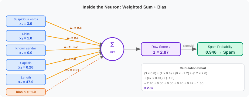
Suppose we have a very simple model with one neuron. It stores one weight for each input feature:
| Feature | Weight | Meaning |
|---|---|---|
| Suspicious words | 0.8 | pushes spam score up |
| Links | 0.6 | pushes spam score up |
| Known sender | -1.2 | pushes spam score down |
| Capital letters | 2.0 | pushes spam score up strongly |
| Message length | 0.01 | barely matters |
The weights can be written as a tensor:
weights = torch.tensor([
    0.8,
    0.6,
   -1.2,
    2.0,
    0.01
])
There is also a bias:
bias = torch.tensor(-1.0)
Think of the bias as the neuron’s default starting mood. Before the model looks at any email features, it starts with a small score. A negative bias means the model begins slightly sceptical of spam; a positive bias means it begins slightly suspicious. The bias is another number the model learns during training, just like the weights.
A positive weight pushes the spam score upward. A negative weight pushes it downward. A larger absolute value means the feature has a stronger effect.
Memory trick: Weights are volume knobs. A high positive weight turns the spam signal up; a negative weight turns it down.
Now that we have the importance score for every feature, we can apply them to a real email and see what score the neuron produces.
7. What calculation does the neuron perform?
For our email:
x = [3, 1, 0, 0.20, 47]
w = [0.8, 0.6, -1.2, 2.0, 0.01]
The neuron multiplies matching positions and adds the results:
| Feature | Calculation | Result |
|---|---|---|
| Suspicious words | 3 × 0.8 | 2.40 |
| Links | 1 × 0.6 | 0.60 |
| Known sender | 0 × -1.2 | 0.00 |
| Capital letters | 0.20 × 2.0 | 0.40 |
| Message length | 47 × 0.01 | 0.47 |
| Bias | -1.00 |
Total: 2.40 + 0.60 + 0.00 + 0.40 + 0.47 - 1.00 = 2.87
The result is called the raw score: z = 2.87.
In PyTorch:
z = email @ weights + bias
The @ operation performs the matching multiplication and addition. It is equivalent to:
z = (
    email[0] * weights[0]
    + email[1] * weights[1]
    + email[2] * weights[2]
    + email[3] * weights[3]
    + email[4] * weights[4]
    + bias
)
So there is no mystery inside the neuron. It is a small calculator.
8. Why is 2.87 not yet the prediction?
The raw score can be any number: -10, -2.3, 0, 1.8, 27. But for spam classification, we want something understandable: a probability between 0 and 1.
For example:
- 0.05 = 5% probability of spam
- 0.70 = 70% probability of spam
- 0.98 = 98% probability of spam
That is where the activation function is used.
9. What does the activation function actually do?
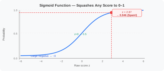
For binary classification, the final activation is usually sigmoid:
probability = torch.sigmoid(z)
Sigmoid is a mathematical operation:
sigmoid(z) = 1 / (1 + e⁻ᶻ)
You do not need to mentally calculate that formula every time. Its behaviour is more important:
| Raw score | Sigmoid result |
|---|---|
| -5 | 0.007 |
| -2 | 0.119 |
| 0 | 0.500 |
| 2 | 0.881 |
| 5 | 0.993 |
Large negative → close to 0. Zero → exactly 0.5. Large positive → close to 1.
For our score z = 2.87, sigmoid produces approximately 0.946. So the model says: spam probability = 94.6%.
Memory trick: Sigmoid is like a thermometer that only reads between 0 and 1, no matter how hot or cold the input is.
10. Probability and prediction are not exactly the same
The model first produces a probability:
0.946
Then the application chooses a threshold:
If probability ≥ 0.5 → spam
Otherwise             → not spam
So 0.946 ≥ 0.5 gives the final prediction: Spam.
There are three separate things:
| Raw score | Probability | Prediction |
|---|---|---|
| 2.87 | 0.946 | Spam |
The model produces the score and probability. The application converts the probability into a business decision. The threshold does not always have to be 0.5. For a security system, we might use probability ≥ 0.30 because missing a dangerous email may be more costly than reviewing a safe one.
11. The complete simple model
import torch

# One email represented by five numerical features
email = torch.tensor([
    3.0,    # suspicious word count
    1.0,    # link count
    0.0,    # sender known: no
    0.20,   # capital-letter percentage
    47.0    # message length
])

# Numbers learned by the model during training
weights = torch.tensor([
    0.8,
    0.6,
   -1.2,
    2.0,
    0.01
])

bias = torch.tensor(-1.0)

# Step 1: produce a raw score
raw_score = email @ weights + bias

# Step 2: turn the score into a probability
spam_probability = torch.sigmoid(raw_score)

# Step 3: turn the probability into a decision
prediction = (
    "spam"
    if spam_probability >= 0.5
    else "not spam"
)

print("Raw score:", raw_score.item())
print("Spam probability:", spam_probability.item())
print("Prediction:", prediction)
The chain is:
Real email
    ↓
Extract measurable information
    ↓
Convert it into numbers
    ↓
Store numbers in a tensor
    ↓
Multiply by learned weights
    ↓
Add bias
    ↓
Produce raw score
    ↓
Apply sigmoid
    ↓
Produce probability
    ↓
Apply decision threshold
    ↓
Spam or not spam
12. Where did the weights come from?
We manually chose weights for this demonstration. A real neural network learns them from labelled examples.
Training data might look like this:
| Suspicious words | Links | Known sender | Capitals | Length | Correct answer |
|---|---|---|---|---|---|
| 5 | 4 | 0 | 0.40 | 31 | 1 |
| 0 | 0 | 1 | 0.02 | 85 | 0 |
| 3 | 2 | 0 | 0.25 | 42 | 1 |
| 0 | 1 | 1 | 0.01 | 110 | 0 |
The correct answer is also converted into numbers:
- Spam = 1
- Not spam = 0
In PyTorch:
labels = torch.tensor([
    [1.0],
    [0.0],
    [1.0],
    [0.0]
])
At first, the model’s weights are random, so predictions may be poor. The model calculates the loss — how far the prediction is from the correct answer. Then backpropagation calculates how each weight contributed to the mistake. The optimizer changes the weights slightly:
Old weight → calculate blame → small adjustment → new weight
This process repeats across many emails until the weights become useful for distinguishing spam from normal email.
Memory trick: Training is like adjusting guitar strings. Each string is a weight; the loss is the out-of-tune sound; the optimizer tightens or loosens each string.
13. What does a hidden layer add?
One input, many neurons
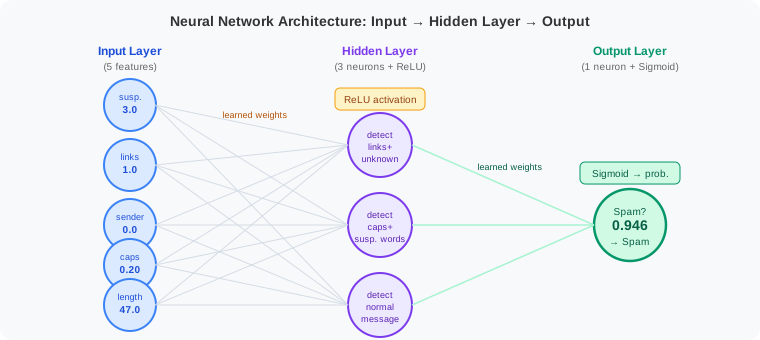
So far we have used one neuron. It received all five features and produced one spam score. But what if we use several neurons at the same time?
Every neuron receives the same five input features. The difference is that each neuron has its own set of weights and its own bias. Think of it as asking several judges the same question, but each judge cares about different evidence.
Each neuron is completely independent:
- Weights: Each neuron has its own five weights. They start random and are learned during training.
- Bias: Each neuron also has its own bias. It is learned independently too.
- Why different? Because we want each neuron to detect a different pattern. If every neuron had the same weights and bias, they would all compute the same score and the hidden layer would be useless.
Who decides how many neurons there are?
The number of neurons in a layer is chosen by the person designing the model. It is part of the architecture, not something the model learns automatically. Common choices are 8, 16, 32, 64, or 128 neurons per hidden layer. A larger number means the model can learn more complex patterns, but it also needs more data and more computation.
For our small spam example, 3 neurons is enough to show the idea. For a real spam classifier with hundreds of input features, you might use 64 or 128 neurons in a hidden layer.
For example, with three neurons:
Neuron 1 weights: [0.8, 0.6, -1.2, 2.0, 0.01]   → responds to spam signals
Neuron 2 weights: [-0.5, 0.2, 1.5, 0.1, 0.05]   → responds to safe-sender signals
Neuron 3 weights: [0.3, 1.2, -0.4, 0.8, 0.00]   → responds to many links
All three neurons see the same email [3, 1, 0, 0.20, 47], but because their weights are different, they produce three different scores. The first neuron might say “likely spam,” the second “looks safe,” and the third “too many links.” Together they capture more nuance than a single neuron can.
Hidden layer + ReLU
A hidden layer is just a group of such neurons placed between the input and the final decision. Each hidden neuron receives the same inputs but has different weights:
- Neuron 1 may respond strongly to: many links + unknown sender
- Neuron 2 may respond strongly to: many capitals + suspicious words
- Neuron 3 may respond strongly to: known sender + long normal message
After each hidden neuron computes its weighted sum, we apply an activation function called ReLU (Rectified Linear Unit). ReLU is a simple rule: keep positive numbers as they are, and turn negative numbers into zero.
ReLU(x) = max(0, x)
Why do we need this? Without an activation function, the hidden layer would just be another weighted sum, and the whole network would still behave like a single neuron. ReLU introduces a non-linear “switch” that lets the model learn richer patterns. It is one of the most common activation functions in deep learning.
Suppose the hidden layer produces raw scores [2.4, -0.7, 1.3]. Applying ReLU:
ReLU([2.4, -0.7, 1.3]) = [2.4, 0.0, 1.3]
That new tensor is passed to the output layer. The model creates a chain:
Original features
    ↓
Learned combinations
    ↓
More learned combinations
    ↓
Final spam score
    ↓
Probability
The hidden layer allows the model to learn combinations rather than considering every feature only in isolation.
Memory trick: A hidden layer is like a team of detectives. Each detective looks at the same clues but notices different patterns.
14. What is permanently stored in the model?
In PyTorch, the same model we just described can be written in a few lines:
import torch.nn as nn

model = nn.Sequential(
    nn.Linear(5, 3),   # 5 input features → 3 hidden neurons
    nn.ReLU(),         # activation: keep positives, zero negatives
    nn.Linear(3, 1)    # 3 hidden neurons → 1 output neuron
)
What does nn.Linear(5, 3) mean?
nn.Linear creates a layer where every input is connected to every output by a weight.
- The first number is how many inputs arrive at the layer.
- The second number is how many neurons live in the layer.
So nn.Linear(5, 3) means: take 5 input numbers and produce 3 output numbers. Each of the 3 neurons receives all 5 inputs, so each neuron has 5 weights. With 3 neurons, that is 3 × 5 = 15 weights. Each neuron also has 1 bias, giving 3 biases.
The second layer nn.Linear(3, 1) takes the 3 hidden values and produces 1 final spam score. It has 1 × 3 = 3 weights and 1 bias.
Why does ReLU have no weights?
ReLU is not a learning layer. It is an operation that runs on the output of the first layer: it keeps positive numbers and turns negative numbers into zero. There is nothing for the model to memorise there, so it has no weight or bias.
Inspecting what the model stores
PyTorch keeps every learnable number in model.parameters(). You can print their names and shapes:
for name, parameter in model.named_parameters():
    print(name, parameter.shape)
Possible output:
0.weight torch.Size([3, 5])
0.bias   torch.Size([3])
2.weight torch.Size([1, 3])
2.bias   torch.Size([1])
The names 0 and 2 come from the position in nn.Sequential. Layer 0 is the first nn.Linear, layer 1 is nn.ReLU (no parameters, so it is skipped), and layer 2 is the second nn.Linear. The shapes show how many numbers are stored in each tensor.
| Name | Shape | Meaning |
|---|---|---|
0.weight |
[3, 5] |
3 hidden neurons, each with 5 weights |
0.bias |
[3] |
1 bias for each of the 3 hidden neurons |
2.weight |
[1, 3] |
1 output neuron with 3 weights |
2.bias |
[1] |
1 bias for the output neuron |
These weights and biases are the only things the model learns and keeps after training. They are the model’s memory.
Memory trick: Think of the architecture as the recipe and the weights as the trained taste. The recipe is code; the taste is the learned state.
15. A slightly more realistic PyTorch model
import torch
import torch.nn as nn

model = nn.Sequential(
    nn.Linear(5, 3),  # 5 email features → 3 hidden values
    nn.ReLU(),        # remove negative hidden signals
    nn.Linear(3, 1),  # 3 hidden values → 1 spam score
    nn.Sigmoid()      # spam score → probability
)

email = torch.tensor([[
    3.0, 1.0, 0.0, 0.20, 47.0
]])

probability = model(email)
prediction = (
    "spam"
    if probability.item() >= 0.5
    else "not spam"
)

print("Probability:", probability.item())
print("Prediction:", prediction)
Notice the double brackets [[3.0, 1.0, 0.0, 0.20, 47.0]]. Its shape is 1 email × 5 features:
print(email.shape) # torch.Size([1, 5])
PyTorch layers normally expect a batch dimension, even when predicting only one example.
16. What does the model really “know”?
It does not store a sentence like “Unknown senders with suspicious words are probably spam.” Instead, that behaviour is distributed across numerical weights. One weight might increase the score for suspicious words; another might reduce the score for a known sender. Hidden neurons might detect combinations of features.
The model’s knowledge is not a collection of readable rules. It is a numerical configuration that produces useful outputs when inputs pass through it.
17. Common mistakes
| Mistake | Why it happens | Fix |
|---|---|---|
| Forgetting the batch dimension | PyTorch layers expect (batch, features) |
Use [[...]] or reshape |
| Forgetting the bias | Bias shifts the decision boundary | Always include + b |
| Using sigmoid in hidden layers | Sigmoid can cause vanishing gradients | Use ReLU in hidden layers |
| Confusing raw score with probability | Raw score can be any number; probability is 0 to 1 | Apply sigmoid for binary output |
| Thinking one neuron is enough | A single neuron is a linear model | Use hidden layers for combinations |
18. Quick review
| Term | What it is | Memory trick |
|---|---|---|
| Tensor | A structured container of numbers | A lunchbox with labelled compartments |
| Feature vector | One row of numbers describing one example | A single email’s numbers |
| Weight | How strongly a feature affects the score | A volume knob |
| Bias | A starting adjustment | The neuron’s default mood |
| Raw score | Sum of weighted inputs plus bias | The pre-decision number |
| Sigmoid | Turns any score into a 0-to-1 probability | A thermometer with a 0-to-1 scale |
| ReLU | Removes negative hidden signals | A bouncer that blocks negatives |
| Hidden layer | Neurons that learn feature combinations | A team of detectives |
| Forward pass | Input → calculations → output | The email travelling through the machine |
| Parameters | Weights and biases the model learns | The trained taste of the recipe |
19. Try it yourself
import torch
import torch.nn as nn

# 1. Create an email tensor with shape (1, 5)
email = torch.tensor([[
    5.0,   # suspicious words
    4.0,   # links
    0.0,   # known sender
    0.40,  # capitals
    31.0   # length
]])

# 2. Build a model with one hidden layer
model = nn.Sequential(
    nn.Linear(5, 3),
    nn.ReLU(),
    nn.Linear(3, 1),
    nn.Sigmoid()
)

# 3. Predict
probability = model(email)
print("Spam probability:", probability.item())

# 4. Inspect the learned parameters
for name, param in model.named_parameters():
    print(name, param.shape)
Final mental model
- Why convert to numbers? Because neural networks perform mathematical operations.
- What is a tensor? A structured box containing those numbers.
- What is a neuron? A small calculator that multiplies inputs by weights, adds them, and adds a bias.
- What are weights? Learned numbers controlling how strongly each signal affects the result.
- What is bias? A learned starting adjustment.
- What is activation? A mathematical transformation applied to a raw result.
- What is a hidden layer? Several calculators learning useful combinations of signals.
- What is stored permanently? Weights and biases.
- What is stored temporarily? Inputs, raw scores, activations, and predictions.
- What does the model predict? A number, probability, or category.
A neural network is not a mysterious digital brain. It is a structured chain of numerical transformations:
Meaningful real-world information
→ numbers
→ tensors
→ learned calculations
→ transformed signals
→ probability
→ decision