
06. Logistic Regression - Introduction
Logistic Regression - Complete Beginner’s Guide 🎯
Welcome! 🚀
Hi! If you’ve already learned Linear Regression, you’re going to love Logistic Regression!
The big difference:
- Linear Regression → Predicts numbers (price, temperature, weight)
- Logistic Regression → Predicts categories (yes/no, spam/not spam, win/lose)
This tutorial assumes zero prior knowledge and will take you from beginner to confident user!
Table of Contents
- What is Logistic Regression?
- Real-World Examples
- The Sigmoid Function (The Magic!)
- How Logistic Regression Works
- The Decision Boundary
- Cost Function & Training
- Evaluation Metrics
- Multi-Class Classification
- Python Examples
- Common Problems & Solutions
1. What is Logistic Regression?
🎯 The Simple Idea
Logistic Regression answers YES/NO questions using probability.
It looks at your data and says:
“There’s an 80% chance this email is spam” “There’s a 30% chance this person will click the ad” “There’s a 95% chance this tumor is benign”
Then we make a decision based on the probability!
🤔 Wait, “Regression” but it’s Classification?
Confusing name alert! 😅
Despite the name “regression”, Logistic Regression is used for classification (predicting categories).
Why “regression”? Because it uses regression techniques internally to calculate probabilities, then converts them to classes.
📊 Linear vs Logistic - Visual Comparison
Linear Regression predicts continuous values:
House Size → Price
2000 sq ft → $400,000
3000 sq ft → $600,000
4000 sq ft → $800,000
Logistic Regression predicts probability of a class:
Email contents → Spam? (Yes/No)
"Buy now! Limited offer!" → 95% spam → YES
"Hi, how are you?" → 5% spam → NO
"Meeting at 3pm" → 2% spam → NO
2. Real-World Examples
📧 Example 1: Email Spam Detection
Input features:
- Number of suspicious words
- Sender reputation
- Has attachments?
- Time of day sent
Output: Spam (1) or Not Spam (0)
🏥 Example 2: Disease Diagnosis
Input features:
- Age
- Blood pressure
- Cholesterol level
- Smoking habits
Output: Has heart disease (1) or doesn’t (0)
💳 Example 3: Credit Card Fraud
Input features:
- Transaction amount
- Location
- Time
- Merchant type
Output: Fraud (1) or Legitimate (0)
📱 Example 4: Click Prediction
Input features:
- User age
- Past click history
- Ad type
- Time of day
Output: Will click (1) or Won’t click (0)
🎓 Example 5: Student Pass/Fail
Input features:
- Hours studied
- Previous grades
- Attendance rate
- Practice problems done
Output: Will pass (1) or fail (0)
3. The Sigmoid Function (The Magic!)
🎯 The Problem with Linear Regression for Classification
What if we tried to use Linear Regression for “Will pass exam?”
Hours Studied → Pass?
1 hour     → ?
5 hours    → ?
10 hours   → ?
100 hours  → ?
Linear Regression gives values like:
- 1 hour → 0.1 (10% probability) ✅
- 5 hours → 0.5 (50% probability) ✅
- 10 hours → 0.9 (90% probability) ✅
- 100 hours → 9.0 ❌ (900%? That’s impossible!)
The problem: Probabilities must be between 0 and 1!
✨ Enter the Sigmoid Function
The Sigmoid function is a magical S-shaped curve that squishes any number into a value between 0 and 1!
Formula:
σ(z) = 1 / (1 + e^(-z))

Where:
- z = any number (can be -∞ to +∞)
- e = mathematical constant (~2.718)
- σ(z) = always between 0 and 1
📊 What the Sigmoid Looks Like
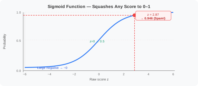
At z = 0, the sigmoid outputs exactly 0.5 — the model is completely uncertain. As z moves further from 0 in either direction, the curve flattens out toward 0 or 1, meaning the model becomes increasingly confident.
🎯 Key Properties
| Input (z) | Output (σ(z)) | Meaning |
|---|---|---|
| -∞ | 0 | Definitely class 0 |
| -3 | 0.05 | 5% chance class 1 |
| -1 | 0.27 | 27% chance class 1 |
| 0 | 0.5 | Uncertain |
| 1 | 0.73 | 73% chance class 1 |
| 3 | 0.95 | 95% chance class 1 |
| +∞ | 1 | Definitely class 1 |
💡 Simple Sigmoid Examples
Calculate σ(z) for different values:
import numpy as np

def sigmoid(z):
    return 1 / (1 + np.exp(-z))

# Examples
print(sigmoid(-3))  # 0.047  (very low probability)
print(sigmoid(0))   # 0.500  (50/50 chance)
print(sigmoid(2))   # 0.880  (88% probability)
print(sigmoid(5))   # 0.993  (99% probability)
🍫 Real-World Analogy: The Confidence Meter
Think of sigmoid as a confidence meter:
Input score:    -10        0        +10
Confidence:    "Definitely  "Maybe  "Definitely
                Not"        could    YES!"
                            be"

Probability:    0%          50%       100%
The further from 0, the more confident the model is!
4. How Logistic Regression Works
🎯 The Two-Step Process
Step 1: Calculate a Linear Combination (just like Linear Regression!)
z = β₀ + β₁×x₁ + β₂×x₂ + ... + βₙ×xₙ
Step 2: Apply Sigmoid to Convert to Probability
P(y=1) = σ(z) = 1 / (1 + e^(-z))
📊 Visual: The Complete Flow
   Features (x)
     ↓
  ┌─────────────────┐
  │ Linear Combine  │   z = β₀ + β₁x₁ + β₂x₂...
  │  (any number)   │
  └─────────────────┘
     ↓ z = 2.5 (example)
  ┌─────────────────┐
  │  Sigmoid σ(z)   │   Squishes to 0-1
  │  (probability)  │
  └─────────────────┘
     ↓ σ(2.5) = 0.92
  ┌─────────────────┐
  │ Decision Rule   │   If > 0.5 → Class 1
  │                 │   Else → Class 0
  └─────────────────┘
     ↓
  Class 1 (Yes!) ✅
🎓 Concrete Example: Customer Churn Prediction �
Predict if a telecom/SaaS customer will cancel their subscription (“churn”) based on how many months they’ve been a customer.
Why does this matter? It costs 5× more to acquire a new customer than to retain an existing one. Companies want to identify at-risk customers BEFORE they leave.
Let’s say we trained the model on past customer data and got:
β₀ = 4 (intercept)
β₁ = -0.5 (coefficient for tenure_months)
So the equation is:
z = 4 - 0.5 × tenure_months
P(churn) = σ(z) = 1 / (1 + e^(-z))
Note: Coefficient is negative → longer tenure = LOWER churn probability (loyal customers stay!)
Predictions for different customers:
| Tenure (months) | z = 4 - 0.5t | σ(z) | P(churn) | Prediction |
|---|---|---|---|---|
| 1 (brand new) | 3.5 | 0.971 | 97% | � Will churn |
| 4 (still new) | 2.0 | 0.881 | 88% | � Will churn |
| 8 (settling in) | 0 | 0.500 | 50% | 🤔 At risk |
| 12 (loyal) | -2.0 | 0.119 | 12% | ✅ Will stay |
| 24 (very loyal) | -8.0 | 0.0003 | 0.03% | ✅ Will stay |
Notice: At 8 months, probability is exactly 50%! This is the decision boundary.
Business action: Target customers with P(churn) > 70% with retention offers (discounts, calls, upgrades).
5. The Decision Boundary
🎯 What is a Decision Boundary?
The decision boundary is the line (or surface) that separates classes.
Default rule: If P(y=1) ≥ 0.5 → Class 1, else Class 0
This happens when z = 0 (since σ(0) = 0.5)
📊 Visualizing the Boundary
For 1 feature (tenure in months):
              CHURN ZONE       LOYAL ZONE
                 ↓                ↓
              ────●────────●─────●─────
              1    4       8    12    24
                          ↑
                  Decision Boundary
                  (z = 0, P = 0.5)
For 2 features (Tenure + Monthly Charges):

The line is the boundary where the model is uncertain (50/50).
🎚️ Adjusting the Threshold
The default threshold is 0.5, but you can change it!
Why change it?
Cancer Detection (Hospital):
- Better to flag healthy people as sick (false alarm) than miss real cases
- Set threshold = 0.3 (more sensitive)
- “Even 30% chance of cancer? Investigate!”
Spam Filter:
- Better to let some spam through than block legitimate emails
- Set threshold = 0.8 (more specific)
- “Only block if 80%+ sure it’s spam”
# Custom threshold example
probabilities = model.predict_proba(X_test)[:, 1]

# Default (0.5)
predictions_default = (probabilities >= 0.5).astype(int)

# Custom (0.3 - more sensitive)
predictions_sensitive = (probabilities >= 0.3).astype(int)

# Custom (0.8 - more specific)
predictions_specific = (probabilities >= 0.8).astype(int)
6. Cost Function & Training
🎯 Why Not Use MSE (like Linear Regression)?
Mean Squared Error doesn’t work well for Logistic Regression!
Why? It creates a non-convex cost function (lots of local minima), making it hard to find the best solution.
✨ The Solution: Log Loss (Cross-Entropy)
Log Loss is the cost function for Logistic Regression!
Formula:
Cost = -[y × log(p) + (1-y) × log(1-p)]

Where:
y = actual class (0 or 1)
p = predicted probability
🤯 What This Actually Means
Two cases:
Case 1: Actual = 1 (true class is “Will Churn”)
Cost = -log(p)

If p = 0.9 (correct, high confidence): Cost = 0.10 ✅ (small)
If p = 0.5 (uncertain):                Cost = 0.69 (medium)
If p = 0.1 (wrong, high confidence):   Cost = 2.30 ❌ (large!)
Case 2: Actual = 0 (true class is “Will Stay”)
Cost = -log(1-p)

If p = 0.1 (correct, low chance):      Cost = 0.10 ✅ (small)
If p = 0.5 (uncertain):                Cost = 0.69 (medium)
If p = 0.9 (wrong, very wrong!):       Cost = 2.30 ❌ (large!)
💡 Key Insight
Log Loss punishes confident wrong answers HEAVILY!
| Predicted Prob | Actual | Cost |
|---|---|---|
| 0.99 | 1 | 0.01 ✅ |
| 0.51 | 1 | 0.67 ⚠️ |
| 0.01 | 1 | 4.61 💀 |
If you say “99% sure” and you’re wrong → BIG penalty!
🏋️ Training (Just Use Gradient Descent!)
The model finds best β values using gradient descent (same as Linear Regression):
1. Start with random β values
2. Calculate predictions using sigmoid
3. Calculate Log Loss
4. Adjust β to reduce Log Loss
5. Repeat until Log Loss is minimized
No need to do this by hand! Sklearn handles it:
from sklearn.linear_model import LogisticRegression

model = LogisticRegression()
model.fit(X, y)  # Done!
7. Evaluation Metrics
🎯 Don’t Just Use Accuracy!
Accuracy = correct predictions / total predictions
Sounds great, right? WRONG!
The Trap (Imbalanced Data):
Dataset: 990 not-spam, 10 spam emails
Bad model: Always predicts "not spam"
Accuracy: 990/1000 = 99% 🎉

But it caught 0% of spam! ❌
Need better metrics!
📊 The Confusion Matrix
The foundation of classification metrics:
                    PREDICTED
                  Class 0  Class 1
              ┌──────────┬──────────┐
ACTUAL  Class 0│  TN  ✅  │  FP  ❌  │
              ├──────────┼──────────┤
        Class 1│  FN  ❌  │  TP  ✅  │
              └──────────┴──────────┘

TP (True Positive):  Predicted YES, actually YES ✅
TN (True Negative):  Predicted NO, actually NO ✅
FP (False Positive): Predicted YES, actually NO ❌ (false alarm!)
FN (False Negative): Predicted NO, actually YES ❌ (missed!)
📊 Important Metrics
1. Accuracy
Accuracy = (TP + TN) / Total

Use when: Classes are balanced
2. Precision
Precision = TP / (TP + FP)

"Of the YES predictions, how many were actually YES?"
Use when: False alarms are costly (spam filter)
3. Recall (Sensitivity)
Recall = TP / (TP + FN)

"Of the actual YES cases, how many did we catch?"
Use when: Missing cases is costly (cancer detection)
4. F1 Score
F1 = 2 × (Precision × Recall) / (Precision + Recall)

Balance between Precision and Recall
Use when: Need both, classes imbalanced
5. ROC-AUC
ROC = Receiver Operating Characteristic
AUC = Area Under the Curve

Range: 0 to 1
- 0.5 = Random guessing
- 0.7 = Decent
- 0.8 = Good
- 0.9 = Excellent
- 1.0 = Perfect
🎯 Real Example: Cancer Detection
Suppose we have 100 patients (10 actually have cancer, 90 don’t):
Confusion Matrix:
                  Predicted
                  No    Yes
              ┌──────┬──────┐
ACTUAL    No  │  85  │   5  │  ← 5 false alarms
              ├──────┼──────┤
          Yes │   2  │   8  │  ← 2 missed cases!
              └──────┴──────┘

Accuracy  = (85+8)/100 = 93%
Precision = 8/(8+5)    = 62% (Of YES predictions, 62% were correct)
Recall    = 8/(8+2)    = 80% (Caught 80% of actual cancer cases)
F1 Score  = 2×(0.62×0.80)/(0.62+0.80) = 70%
For cancer detection, we want HIGH RECALL (don’t miss cases!)
8. Multi-Class Classification
🎯 What if We Have More Than 2 Classes?
Examples:
- Image: cat, dog, bird, fish, horse
- Sentiment: positive, neutral, negative
- Iris flower: setosa, versicolor, virginica
📊 Two Strategies
Strategy 1: One-vs-Rest (OvR)
Train one binary classifier per class:
Classifier 1: "Cat vs (Dog, Bird, Fish)"
Classifier 2: "Dog vs (Cat, Bird, Fish)"
Classifier 3: "Bird vs (Cat, Dog, Fish)"
Classifier 4: "Fish vs (Cat, Dog, Bird)"

Final answer: Class with highest probability
Strategy 2: Multinomial (Softmax)
Single model that calculates probability for ALL classes at once:
Output: [P(cat), P(dog), P(bird), P(fish)]
Sum = 1
Pick class with highest probability
🛠️ Python Implementation
from sklearn.linear_model import LogisticRegression

# One-vs-Rest (default)
model_ovr = LogisticRegression(multi_class='ovr')

# Multinomial (softmax)
model_multi = LogisticRegression(multi_class='multinomial')

# Both work the same way
model_ovr.fit(X_train, y_train)
predictions = model_ovr.predict(X_test)
probabilities = model_ovr.predict_proba(X_test)
9. Python Examples
🎓 Complete Example: Customer Churn Prediction �
import numpy as np
import pandas as pd
import matplotlib.pyplot as plt
from sklearn.linear_model import LogisticRegression
from sklearn.model_selection import train_test_split
from sklearn.metrics import (
    accuracy_score, precision_score, recall_score,
    f1_score, confusion_matrix, classification_report
)

# Step 1: Create customer dataset
np.random.seed(42)
n_customers = 300

# Features for each customer:
#   - tenure_months: how long they've been a customer
#   - monthly_charges: how much they pay per month
tenure_months = np.random.uniform(1, 36, n_customers)
monthly_charges = np.random.uniform(20, 120, n_customers)

# True relationship (with noise):
#   - Short tenure + high charges → more likely to churn
score = 4 - 0.2*tenure_months + 0.04*monthly_charges + np.random.normal(0, 1, n_customers)
churned = (score > 0).astype(int)

df = pd.DataFrame({
    'tenure_months': tenure_months.round(1),
    'monthly_charges': monthly_charges.round(2),
    'churned': churned
})

print("📊 Customer Dataset:")
print(df.head())
print(f"\nTotal customers: {len(df)}")
print(f"Churned:  {df['churned'].sum()}  ({df['churned'].mean()*100:.1f}%)")
print(f"Retained: {len(df) - df['churned'].sum()}  ({(1-df['churned'].mean())*100:.1f}%)")

# Step 2: Split data
X = df[['tenure_months', 'monthly_charges']]
y = df['churned']

X_train, X_test, y_train, y_test = train_test_split(
    X, y, test_size=0.2, random_state=42
)

# Step 3: Train model
model = LogisticRegression()
model.fit(X_train, y_train)

print("\n📋 Model Coefficients:")
print(f"Intercept (β₀): {model.intercept_[0]:.3f}")
for feature, coef in zip(X.columns, model.coef_[0]):
    print(f"  {feature}: {coef:.3f}")

print("\n💡 Interpretation:")
print("  - tenure_months coef NEGATIVE → longer tenure = less churn (loyal!) ✅")
print("  - monthly_charges coef POSITIVE → higher charges = more churn ⚠️")

# Step 4: Make predictions
predictions = model.predict(X_test)
probabilities = model.predict_proba(X_test)

print("\n🔮 Sample Predictions:")
for i in range(5):
    actual = y_test.iloc[i]
    pred = predictions[i]
    prob_churn = probabilities[i][1]
    label = "� WILL CHURN" if pred == 1 else "✅ WILL STAY"
    print(f"  Tenure: {X_test.iloc[i]['tenure_months']:.0f}mo, "
          f"Charges: ${X_test.iloc[i]['monthly_charges']:.0f}, "
          f"P(churn): {prob_churn:.1%}, "
          f"Predicted: {label}, Actual: {actual}")

# Step 5: Evaluate
print("\n📊 Evaluation Metrics:")
print(f"  Accuracy:  {accuracy_score(y_test, predictions):.2%}")
print(f"  Precision: {precision_score(y_test, predictions):.2%}  ← Of flagged churners, how many really churn?")
print(f"  Recall:    {recall_score(y_test, predictions):.2%}  ← Of actual churners, how many did we catch?")
print(f"  F1 Score:  {f1_score(y_test, predictions):.2%}")

# Step 6: Confusion Matrix
print("\n📊 Confusion Matrix:")
cm = confusion_matrix(y_test, predictions)
print(cm)

print("\n📋 Classification Report:")
print(classification_report(y_test, predictions, target_names=['Stayed', 'Churned']))
💡 Why RECALL Matters for Churn Prediction
For customer churn, RECALL is critical:
- Missing a churner = lost revenue forever 💸
- A false alarm just means an unnecessary retention offer (cheap!)
- Better to flag too many at-risk customers than miss real ones
Recommendation: Use a LOWER threshold (e.g., 0.3) to catch more potential churners and intervene early.
📊 Visualizing the Decision Boundary
import matplotlib.pyplot as plt
import numpy as np

# Create mesh grid
x_min, x_max = X['tenure_months'].min() - 1, X['tenure_months'].max() + 1
y_min, y_max = X['monthly_charges'].min() - 5, X['monthly_charges'].max() + 5

xx, yy = np.meshgrid(
    np.linspace(x_min, x_max, 100),
    np.linspace(y_min, y_max, 100)
)

# Predict probabilities for each point
Z = model.predict_proba(np.c_[xx.ravel(), yy.ravel()])[:, 1]
Z = Z.reshape(xx.shape)

# Plot
fig, ax = plt.subplots(figsize=(12, 6))

# Filled contour for probabilities (red = churn zone, green = loyal zone)
contour = ax.contourf(xx, yy, Z, levels=20, cmap='RdYlGn_r', alpha=0.6)
plt.colorbar(contour, label='P(Churn)')

# Decision boundary at 0.5
ax.contour(xx, yy, Z, levels=[0.5], colors='black', linewidths=2)

# Plot data points
ax.scatter(X[y==0]['tenure_months'], X[y==0]['monthly_charges'],
           c='green', label='✅ Stayed (Loyal)', s=80, edgecolors='black')
ax.scatter(X[y==1]['tenure_months'], X[y==1]['monthly_charges'],
           c='red', label='🚨 Churned', s=80, edgecolors='black', marker='X')

ax.set_xlabel('Tenure (months)', fontsize=12)
ax.set_ylabel('Monthly Charges ($)', fontsize=12)
ax.set_title('Customer Churn Decision Boundary', fontsize=14)
ax.legend()
plt.tight_layout()
plt.show()
10. Common Problems & Solutions
❌ Problem 1: Imbalanced Data
Issue: 99% one class, 1% other class
Solutions:
# Option 1: Use class_weight='balanced'
model = LogisticRegression(class_weight='balanced')

# Option 2: Manual weights
model = LogisticRegression(class_weight={0: 1, 1: 10})

# Option 3: Resample the data (SMOTE)
from imblearn.over_sampling import SMOTE
smote = SMOTE()
X_balanced, y_balanced = smote.fit_resample(X_train, y_train)
❌ Problem 2: Features on Different Scales
Issue: Some features 0-1, others 0-10000
Solution: Always scale your features!
from sklearn.preprocessing import StandardScaler

scaler = StandardScaler()
X_train_scaled = scaler.fit_transform(X_train)
X_test_scaled = scaler.transform(X_test)

model.fit(X_train_scaled, y_train)
❌ Problem 3: Overfitting
Issue: Great train accuracy, poor test accuracy
Solution: Use regularization!
# L2 regularization (Ridge-like)
model = LogisticRegression(penalty='l2', C=1.0)

# L1 regularization (Lasso-like, feature selection)
model = LogisticRegression(penalty='l1', solver='liblinear', C=1.0)

# Note: C is INVERSE of regularization
# Smaller C = more regularization
❌ Problem 4: Non-Linear Boundaries
Issue: Data isn’t linearly separable
Solution: Add polynomial features
from sklearn.preprocessing import PolynomialFeatures

poly = PolynomialFeatures(degree=2)
X_poly = poly.fit_transform(X)

model.fit(X_poly, y)
🎓 Summary - Logistic Regression in 5 Bullets
- Predicts probability of class (0 to 1) using sigmoid function
- Threshold of 0.5 by default (adjustable for different needs)
- Log Loss is the cost function (punishes confident wrong answers)
- Multiple metrics matter - not just accuracy (use F1, ROC-AUC)
- Always scale features and consider class imbalance
🎯 Cheat Sheet
# Import
from sklearn.linear_model import LogisticRegression
from sklearn.preprocessing import StandardScaler
from sklearn.metrics import classification_report

# Scale features
scaler = StandardScaler()
X_scaled = scaler.fit_transform(X)

# Train model
model = LogisticRegression(
    penalty='l2',         # Type of regularization
    C=1.0,                # Regularization strength
    class_weight='balanced',  # Handle imbalance
    max_iter=1000         # Iterations
)
model.fit(X_train, y_train)

# Predict
predictions = model.predict(X_test)
probabilities = model.predict_proba(X_test)[:, 1]

# Evaluate
print(classification_report(y_test, predictions))

# Custom threshold
custom_predictions = (probabilities >= 0.3).astype(int)
🚀 Next Steps
After mastering this:
- Regularization Deep Dive - Master Ridge, Lasso, Elastic Net
- Decision Trees - Tree-based classification
- Random Forest - Ensemble of trees
- Support Vector Machines (SVM) - Powerful classifier
- Neural Networks - Logistic regression on steroids!
Happy Classifying! 🎯✨